If you have any questions about the code here, feel free to reach out to me on Twitter or on Reddit.
Shameless Plug Section
If you like Fantasy Football and have an interest in learning how to code, check out our Ultimate Guide on Learning Python with Fantasy Football Online Course. Here is a link to purchase for 15% off. The course includes 15 chapters of material, 14 hours of video, hundreds of data sets, lifetime updates, and a Slack channel invite to join the Fantasy Football with Python community.
Using EDA to Analyze Positional Value
Another April has passed and, although very unique this year, another edition of the NFL Draft has come and gone. Like many years past, we saw a handful of potential franchise-changing Quarterbacks come off of the board immediately. It is afterall the most important position on the field in the NFL. So, why is that not the case in Fantasy Football? We’ll do some Exploratory Data Analysis using Python of positional value to take a look.
If you’ve played a good amount of Fantasy Football you’ve probably come across that newbie (or maybe it was you?) who jumped at their first chance to get Peyton Manning or Patrick Mahomes, but why is this strategy so frowned upon?
In our first chunk of code, we’ll import the Python libraries that will be needed as well as the yearly data from 2010 - 2019 to try to gain some insight. To begin importing the data, we run a for loop that iterates over each year and grabs the .csv from the current directory. The raw data only contains yearly totals, but to account for injuries/missed games, we’re interested in adding a Points Per Game (PPG) column. Additionally, we’ll add a Season column and remove unneeded data before appending each table into df.
Once we have all of the data combined/cleaned up, let’s add a few features. First we’ll need to write a couple of functions; the first function, create_tier will label each player based off of their Z-score for a given season (this will be explained shortly) and the second function, position_tiers will assign each player, per season, a positional tier such as RB1 for the top 10 RBs in a 10-team league.
In this next block of code we’ll calculate mean, standard deviation and z-score based on assumed number of potential starting roster spots; that is, the top 10 QBs, top 30 RBs and WRs and top 20 TEs (1QB, 2RB, 2WR, 1TE, Flex).
What the z-score tells us how many standard deviations from the mean a certain observation is. In a normal distribution, 68% of the data falls within mean +/- 1 standard deviation, 95% within 2 and 99% within 3. Using the z-score allows us to compare each player to his position’s scoring distribution amongst “startable” players.
With this information we now have, we can see the top 15 season performances based on a player being set apart from his position group. Here we see that in 2019, Michael Thomas and CMC were both over 3.5 standard deviations ahead of the mean of the top 30 WRs and RBs respectively.
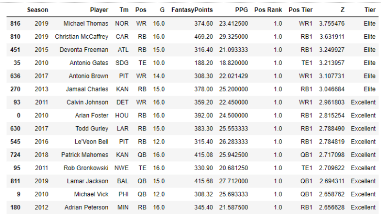
What else is interesting about this? Just 3 QBs barely crack the list even though those 3 seasons were remarkable. The reasoning behind this is simple; when looking at the top 10 QBs, none of them REALLY set themselves apart from the pack. Let’s look at 2019:
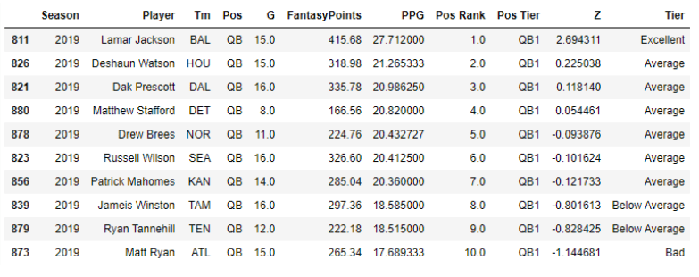
Outside of an historic season from Lamar Jackson, the rest of the QB1s are all within 4 PPG of each other with 2-7 separated by less than 1 point. Now, some of us grabbed Lamar late/for cheap in drafts last year (thanks for the championship, Lamar), but that’s not happening in 2020. Guys like Watson, Wilson and Mahomes will be sprinkled throughout the mid-rounds with just a few PPG added compared to late-rounders.
As for RBs and WRs? Well, remember that you need 2-3 each and each round you pass up on one for a QB, you potentially create a domino effect in hampering your positional depth. The boxplot below shows scoring distribution from 2010 - 2019 per starting roster spot (RB3, WR3 and TE2 represent Flex options).
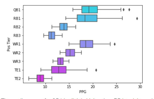
The median score for QB1 is slightly higher than RB1 and the variability is almost the same, but sliding towards that back end of RB1 may snowball into disadvantages at RB2 and RB3 as well (same idea for WRs) that outweigh the gain of taking QBs in that 2-7 range.
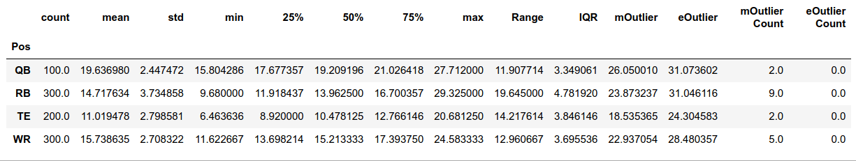
The final piece of code I’ll highlight here is generating a summary statistics table for PPG per position over the last 10 seasons. Included in the table is Interquartile Range (IQR) which helps to determine outliers, Range and Mild and Extreme Outlier values and counts. The key takeaway here again is the demand for RBs and WRs. Yes, the Range is higher for these positions because there are triple the number of players, but everyone NEEDS at least 3 and will likely load up on more for bench depth. Load up early and often if you can, and find the next Jackson or Mahomes at the end (okay, good luck with that one).