If you have any questions about the code here, feel free to reach out to me on Twitter or on Reddit.
Shameless Plug Section
If you like Fantasy Football and have an interest in learning how to code, check out our
Ultimate Guide on Learning Python with Fantasy Football Online Course. Here is a link to purchase for
15% off. The course includes 15 chapters of material, 14 hours of video, hundreds of data sets, lifetime
updates, and a Slack channel invite to join the Fantasy Football with Python community.
This is a remake of part three of the beginner series. If you haven't read part one already, navigate to that through this link here.
In this part of the series, we take a look at how to use real Fantasy Football data and start to use Python to
do the sorts of things we can do in excel.
In this part, we are just going to load in the data and begin a discussion on pandas DataFrames. In the next
couple parts, we are going to loading in 2019 fantasy data and analyzing usage and fantasy performance. After we
load in the data, we are going to filter out all those players who are not running backs. We'll only be working
with running backs for this part of the series. After that, we'll find the "usage" value for each player by
calculating number of targets + number of carries. We'll then be ranking our data to show the usage and fantasy
points rankings for our data in a table that's called a DataFrame (which looks like an excel
spreadsheet).
If you're coming from part 2 and wondering how we do all this, the answer is with libraries. Libraries
are code bases that have been written for us by other people. Remember how last time we wrote a function to
better modularize our code and dealing with repeating patterns? Well a library comes with a set of functions and
classes (more on this in future parts) that we can import and use in our code. We'll be importing
the pandas library for this part of the series, which is a library provides a set of Python objects for dealing
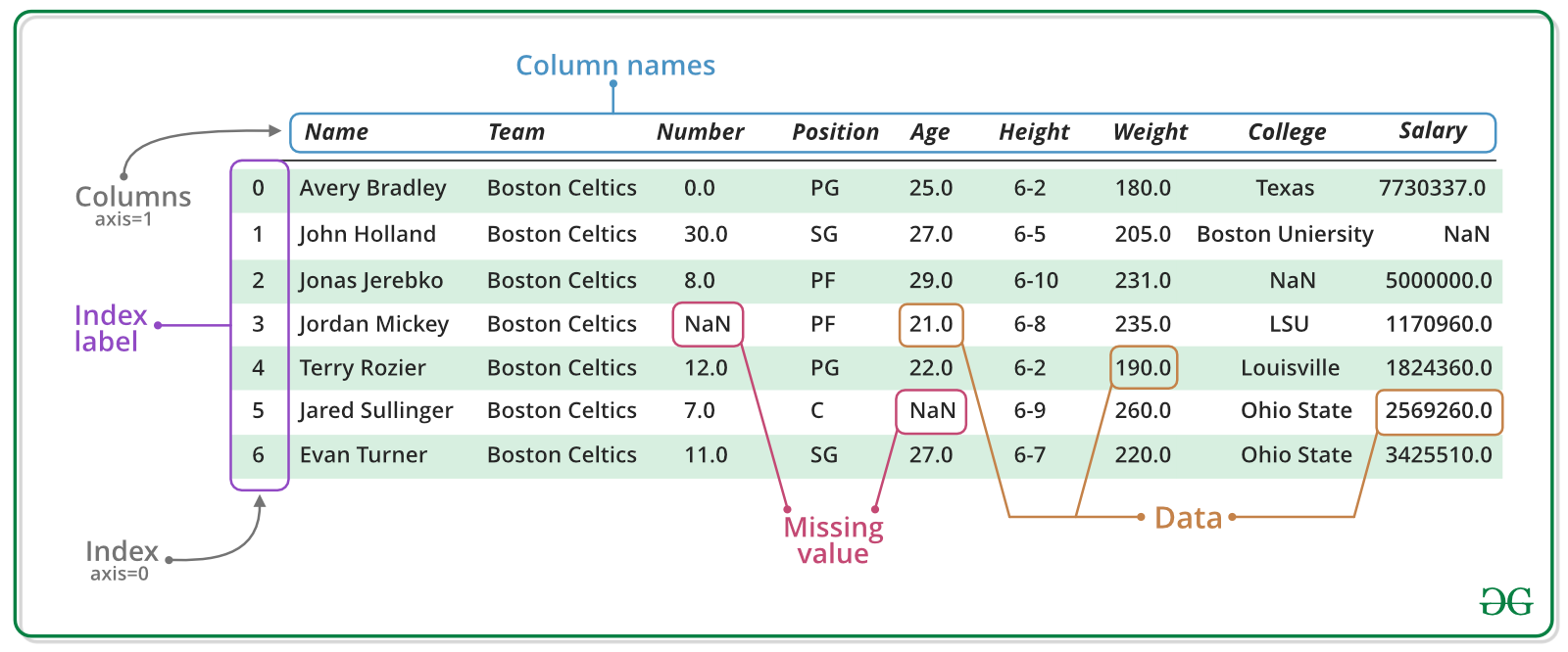
with data. Pandas comes with a function that lets us read a CSV file in to what's called a DataFrame, for
example. A DataFrame looks like this:
Image source: geeksforgeeks.org
If you want to learn more about Pandas, you can read
more in the documentation here.. If you go to the section labeled "API Reference", you can take a look
at all the tools pandas provides for us to work with data. In this part, we won't have to worry about installing
pandas since we are writing our code in Google Colab. Google Colab is meant for data science, and as such,
already has a lot of the popular data science libraries already pre-installed for you.
Finally, download this CSV file
which contains the 2019 data. To be able to use it in Google Colab, you'll need to upload it to Google
Colab. In the side bar of Google Colab, there will be an icon that looks like a folder. This is the files tab.
There might be something that says "Connecting to a runtime to enable file browsing.". This should only last a
few seconds before you are allowed to "Upload". Upload the CSV file you downloaded here and you're good to go.
In the first line, we import the pandas library. import is the Python keyword used to
bring in libraries. We can pull out objects/functions we need from the library using a dot notation.
as tells Python what we'd like to refer our imported library as. In this case, we'd like to refer
to pandas as pd. Throughout our code, if we want to pull a function out from the pandas library,
we'll use the notation pd.function_we_are_bringing_out.
df = pd.read_csv(csv_path)
In this line here, we actually use this dot notation. We are pulling out a function called read_csv
which takes an argument of a string - the file path to our CSV files. In Google Colab, you don't have to worry
about specifying a file path, only the file name. It returns a pandas DataFrame that we can use to do data
analysis on. Here's a link to the documenation page on read_csv - link. We save the
function return value to a variable we call df
Classes and Methods
Like we discussed in previous parts, everything in Python is an object. Each object has a set of attributes and
methods associated with that object. An attribute is a characterstic about an object that we can access using a
dot notation. A method is a process or function we can run on an object also using the dot notation. Moreover,
all objects belong to a certain class. That's all you really need to know for now. Our df variable
is an object of the class DataFrame. Here's some example of some attributes we can access from our
df object.
Using .head()
Now that we've talked about attributes and know a couple, let's talk about methods. Methods are functions that
are "attached" to objects. We'll be going over many more methods as this series continues as methods are an
integral concept to Object Oriented Programming. Python is a Object Oriented Programming language, which means
that everything is defined in terms of classes and objects. And every object has attributes or methods.
Attributes are characteristics that tell us information about our object. In the case of shape, for example, we
were able to see the shape of our DataFrame. In the case of columns, we were able to see our columns. These
attributes are objects as well, with their own class and methods and attributes. I don't want to confuse you if
this is your first time programming and dealing with OOP, so that's all you need to know for now.
Methods, on the other hand, are a set of processes we can run on a object. We call a method using the
dot notation and calling it like we would a function.
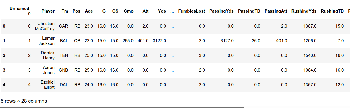
One method, head shows us the first five rows of our DataFrame if we do not provide it an argument
(many functions have default arguments like this). Let's run df.head() and see what we get back. In
a new Google Colab cell, run this one line of code.
Below is what you should have gotten back as an output. That's what a Pandas dataframe
looks like. You can see it looks a lot like a spreadsheet.
Conclusion
So in this part of the series, we were able to load in our spreadsheet. Admittedly, nothing
super exciting so far but we need to build up a basis before doing some actually interesting work. In the next
part of the series, we'll be taking that DataFrame above and sorting by position and finding targets and number
of carries. In that part after that, we'll be creating a new column for usage and ranking our data and seeing
the correlation between running back usage and fantasy points output
In our intermediate series, we talk about this in part one. Most of the variation in
fantasy football output comes down to how often is a player getting touches and targets.
 Photo by Gail Burton, AP