If you have any questions about the code here, feel free to reach out to me on Twitter or on Reddit.
Shameless Plug Section
If you like Fantasy Football and have an interest in learning how to code, check out our
Ultimate Guide on Learning Python with Fantasy Football Online Course. Here is a link to purchase for
15% off. The course includes 15 chapters of material, 14 hours of video, hundreds of data sets, lifetime
updates, and a Slack channel invite to join the Fantasy Football with Python community.
What We'll Be Doing in This Part
In this part of Learn Python with Fantasy Football, we are going to be building upon the
DataFrame we rendered in the last part of the series. If you have not already read part one of the series, here's a link to that
In this part, we are going to be filtering out all those players who are not running backs
and I'll be showing you how to create a new column based off values in other columns in our DataFrame.
In the next part of the series, we will be creating two new columns for "FantasyPoints
Rank" and "Usage Rank" and comparing the two values for each row in our DataFrame. In future, posts, we'll be
examining the relationship between Usage and Fantasy Points more. We'll then be circling back to the DataFrame
we create in part 4/5 of this series and trying to find regression candidates for your 2020 draft.
A Review of Last Time
Last time, recall that we created a DataFrame after importing a CSV file in Google Colab. Recall also that
DataFrames are similar to spreadsheets, in that it is data organized in a collection of rows and columns. In
this part of the series, we will simply be building upon this DataFrame we imported last time.
Step One: Filter Out Unnecessary Columns and Positions
In programming, it is best to break down a problem in to a series of steps. The longer you program, the longer
you'll naturally do this with every problem you encounter. In this case, our problem is two-fold: We want to
filter out all those positions from our DataFrame that are not running back, and we only want to include those
columns essential to calculating our Usage Rank and Fantasy Points Rank columns in the next part.
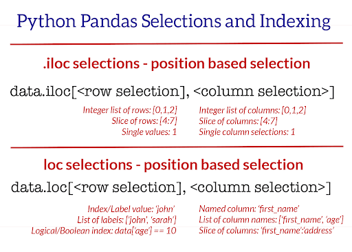
In pandas, we can actually solve this problem in one line using .loc. Below is an image
representation of how .loc works.
In this part of the example, we'll be setting our df variable we created last time equal to itself
with .loc tacked on to df. This will make more sense in a moment. Essentially, we are
going to be "re-setting" our df.
Load the Same Notebook as Last Time
Load up the same notebook as last time (this is important, otherwise this code won't work), and let's get
started
These two lines of code are all that we're going to be writing in this part, but if you're a complete Python
beginner there is a lot of information here for you to digest.
If you refer to the picture above on .loc (ignore .iloc for now, that's a topic for
another day), you'll see that we can select sections of our DataFrame based off row, column values. That's
exactly what we are doing in the first line of our code here. The first part of our code following
.loc[ (df['Pos'] == 'RB') is our "row selector". We are telling pandas that for each
row in our DataFrame, only select those rows where the column value "Pos" is equal to "RB". If the row value for
the column "Pos" is not equal to "RB", do not include it in our new DataFrame. This sort of filtering is known
as Boolean indexing. You can learn more about boolean indexing here.
The second part of our .loc is the column selector. We simply pass in a list of column names we'd
like included in our final DataFrame. We are just telling pandas, "Here are the columns we'd like included,
exclude every column in our original DataFrame that is not in this list". Notice the square brackets. We need to
pass in a list. Do not make the mistake of forgetting to pass in a list and just passing in 4 strings - it won't
work. Pandas needs a list for the column indexer.
One more thing that might be confusing for beginners here is the re-declaration of our df variable
here. All we are doing here is re-setting our df to equal itself plus the
.loc transformation we wrote on it. On the left side of the equation, we have our new and improved
df, the df that only includes running backs and the columns we specified. On the right
side of the equation, when we reference df, we are referencing the old df we created
in part 3 of the series. This concept of re-declaring variables is usually a tough one for beginners to wrap
their heads around. Don't move on to the next part until you've wrapped your head around it. Play around with
the code and try to change up some of the variable names to better understand how it works.
The second line is a bit less complicated. To set a new column in pandas, you simply use the syntax
df['NewColumnName'] = df['ColumnOne'] + df['ColumnTwo'] - df['ColumnThree'] and so on and so on.
You can add and subtract columns together, and pandas will simply take each row, and subtract/add the
corresponding columns. For example, if a row has targets of 20 and carries of 10, the pandas will simply add
these two numbers together in our case and move that new value in to the new column we specified.
Here, we specify Usage as targets + number of carries. I like to use targets as an
indicator of usage as opposed to catches as an indicator of involvement in an offense. Targets always precede
catches (Well, almost always).
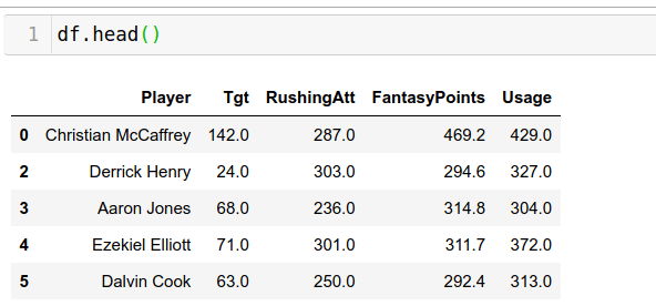
Finally, let's run df.head() and take a look at our new DataFrame.
Conclusions/Takeaways
Not a lot of code in this part of the series, but I hope you learned something new here. I'll be posting these
beginner series posts every Friday for the remainder of the off season. As an exercise to really drill down the
concepts learned here, ahead and try to create new columns other than Usage. As a more difficult challenge, try
going back and using .loc to filter out all those rows that are not WR and only include WR relevant
columns.
In the next part of the series, we'll be examining the ranks of Usage and Fantasy Points and seeing how these
two columns match up. We'll be trying to look for gaps between Usage and Fantasy Points. For example, if a
player is ranked 10th in Usage but 2nd in Fantasy Points - hint: this is actually for the case for one player.
Does this mean this player was extremely efficient with their usage in 2019 or does it mean they are possibly
due for a regression? We'll find out in future parts.
Thanks for reading! You guys are awesome.
 Photo by Lachlan Cunningham, Getty Images