`
If you have any questions about the code here, feel free to reach out to me on Twitter or on Reddit.
Shameless Plug Section
If you like Fantasy Football and have an interest in learning how to code, check out our
Ultimate Guide on Learning Python with Fantasy Football Online Course. Here is a link to purchase for
15% off. The course includes 15 chapters of material, 14 hours of video, hundreds of data sets, lifetime
updates, and a Slack channel invite to join the Fantasy Football with Python community.
Ranking Players
In this part of the beginner series, we are going to begin to look at our DataFrame we created last time a bit
more closely and try to find some regression candidates for the 2020 season. If you have not already read part
one of the series, here's a link for that. Part one of the series
starts you off at the absolute basics of Python. If you want to instead skip ahead to where we start using
Pandas, check out part 3 instead.
We are first going to do this using two Pandas DataFrame methods known as rank and
sort_values. Remember the couple last times we started going over some of our first DataFrame
methods/attributes such as head and columns. rank and
sort_values are both methods and behave similarly to the head method we've used
before.
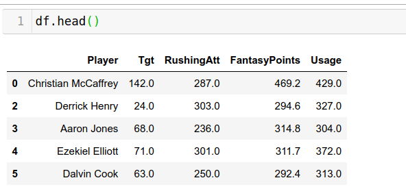
Let's start by bringing in the DataFrame we created last time. Either open the Google Colab Notebook you were
working with last time, or open a new Google Colab notebook to regenerate our DataFrame back to it's current
state.
You should get the output below. If you do not already have access to the 2019 csv file we are importing in to
our code here, here's a download link for
that.
Remember that your CSV file needs to be uploaded to be able to run this code. You may need to re-upload it. In part 4, I give instructions on how to do that.
This is all of the code for this part, and although like last time it does not seem like a lot, it is actually
quite dense if you haven't coded before. We'll go over the output and the DataFrame we get back in just a
minute.
In that first line, we are creating a new column based off another column (Usage) and finding each
player's Usage rank. This method also takes a keyword argument. A keyword argument is an argument that you have
to explicitly define in the functions parameters. If you look ahead to the third line of our code, you'll notice
that head doesn't require a keyword argument. Some arguments in a function have to explicitly
specficied and some arguments can be assumed. We'll get in to the reasons for this in future parts, but it boils
down to the fact that functions can have optional arguments. You can find our which arguments go in which
functions by reading
through the documentation.
In the case of rank, one such argument it takes is ascending. If we specify that
ascending is equal to False, we are telling Pandas that we want to rank the largest
numbers in the column we are ranking higher. CMC had the higher usage numbers and so he gets a 1 for
UsageRank
We repeat the same process for FantasyPoints. We repeat this process becuase we want to find gaps
between Usage and Fantasy Points scored on the season.
Finally, we use another method I talked about called sort_values. This method sorts our DataFrame
by a certain column. By default, it sorts the columns by ascending order (smallest to largest). Since we are
sorting via the rank column, this is exactly what we want. It takes in a keyword argument of by, so
we can tell Pandas which column we'd like to sort on. (It also takes in an argument of ascending,
in case you wanted to sort your DataFrame in descending order of a column. In this case, we don't.)
We then take on head to the end of that last line, because a DataFrame sorted via
sort_values is still a DataFrame. We haven't discussed this previously, but head also
takes in arguments. By default, head gets you back the top 5 rows of a DataFrame (By the way, try
to figure out what running the .tail() method does), but if you specify an argument, that argument
will override it's default of 5. Here, we specify 15, which means get us back the top 15 rows in our DataFrame.
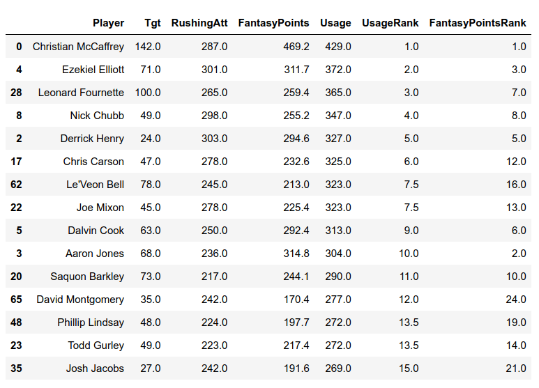
Here is the output from the code we ran above. In the next part, we'll be examining these "gaps" between Usage
and Fantasy Points further and trying to figure out what it means for your 2020 draft. We'll start talking about
the relationship between Usage and Fantasy Points scored and what it means when a player has a low Usage ranking
but high Fantasy output. For now, try to examine the DataFrame and find some gaps between Usage and Fantasy
Points. Two interesting cases that pop out to me are Aaron Jones and David Montgomery. Montgomery had the 12th
highest utilization amongst RBs but finished RB24. On the flip side, Aaron Jones finished 10th in utilization in
RBs but finished RB2. Could this indicate that Aaron Jones is due for a negative regression to the mean and
Montgomery is due for a positive regression to the mean? We'll find out in the next part of this series.
Thanks for reading, you guys are awesome!
 Photo by Evan Habeeb, USA TODAY Sports