If you have any questions about the code here, feel free to reach out to me on Twitter or on Reddit.
Shameless Plug Section
If you like Fantasy Football and have an interest in learning how to code, check out our
Ultimate Guide on Learning Python with Fantasy Football Online Course. Here is a link to purchase for 15%
off. The course includes 15 chapters of material, 14 hours of video, hundreds of data sets, lifetime updates,
and a Slack channel invite to join the Fantasy Football with Python community.
Usage vs. Efficiency
In this part of the beginner series, we are going to introduce a few new concepts. In past
posts, we've worked with the Pandas library, which is primarily used to work with data in the form of DataFrames.
Today we are going to learn about pandas plotting capabilities that allow us to visualize our data in a way that
using .head() or simply outputting our data to the console wouldn't allow us to do. We will be
introducing an additional Python library called matplotlib to help us plot our data. Matplotlib is
Python's de-facto data visualization library and is also included in Google Colab and similar notebook environments,
much like Pandas is.
For those of you who are new to this series, check out part one
here.
Either open up the Google Colab notebook you used last time, or run the following code below
to get you back to where we currently are in the code.
|
Player |
Tgt |
RushingAtt |
FantasyPoints |
Usage |
UsageRank |
FantasyPointsRank |
| 0 |
Christian McCaffrey |
142.0 |
287.0 |
469.2 |
429.0 |
1.0 |
1.0 |
| 4 |
Ezekiel Elliott |
71.0 |
301.0 |
311.7 |
372.0 |
2.0 |
3.0 |
| 28 |
Leonard Fournette |
100.0 |
265.0 |
259.4 |
365.0 |
3.0 |
7.0 |
| 8 |
Nick Chubb |
49.0 |
298.0 |
255.2 |
347.0 |
4.0 |
8.0 |
| 2 |
Derrick Henry |
24.0 |
303.0 |
294.6 |
327.0 |
5.0 |
5.0 |
| 17 |
Chris Carson |
47.0 |
278.0 |
232.6 |
325.0 |
6.0 |
12.0 |
| 62 |
Le'Veon Bell |
78.0 |
245.0 |
213.0 |
323.0 |
7.5 |
16.0 |
| 22 |
Joe Mixon |
45.0 |
278.0 |
225.4 |
323.0 |
7.5 |
13.0 |
| 5 |
Dalvin Cook |
63.0 |
250.0 |
292.4 |
313.0 |
9.0 |
6.0 |
| 3 |
Aaron Jones |
68.0 |
236.0 |
314.8 |
304.0 |
10.0 |
2.0 |
| 20 |
Saquon Barkley |
73.0 |
217.0 |
244.1 |
290.0 |
11.0 |
10.0 |
| 65 |
David Montgomery |
35.0 |
242.0 |
170.4 |
277.0 |
12.0 |
24.0 |
| 48 |
Phillip Lindsay |
48.0 |
224.0 |
197.7 |
272.0 |
13.5 |
19.0 |
| 23 |
Todd Gurley |
49.0 |
223.0 |
217.4 |
272.0 |
13.5 |
14.0 |
| 35 |
Josh Jacobs |
27.0 |
242.0 |
191.6 |
269.0 |
15.0 |
21.0 |
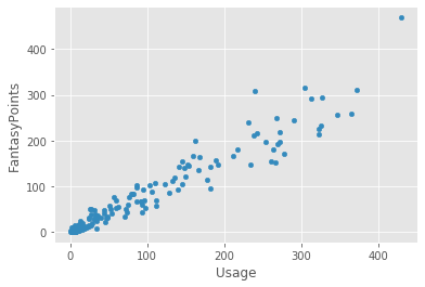
Here we have our top 15 running backs for 2019 in terms of utilization. What we want to do in
this part is visualize the relationship between usage/utilization and Fantasy Football output for running backs
using this entire DataFrame. Spoiler alert: there is a linear relationship between how often a RB is utilized in an
offense and how many Fantasy points he scores for you. What we are tying to get at here is that maybe if a player
strayed far from this relationship, they are due for some sort of regression to the mean (either postive or
negative). This will make a lot more sense once we actually visualize our results.
Awesome, we just created our first visualization in literally three lines of Python code.
Let's run through what happened here.
Introducing matplotlib
In the first line of that block, we imported matplotlib. We had to import a
module (think of a module as a sub-section of a library) from the matplotlib library called
pyplot which we tell Python we'd like to refer to as plt for the rest of our code. This is
exactly how we do import pandas as pd, except right now, instead of importing all of
matplotlib, we want to import just one part, or module, from matplotlib. So we say to
Python "from matplotlib import the pyplot part, and let us refer to pyplot as plt for the rest of our code."
Inside the pyplot module, there is another submodule known as style which is
specifically meant to deal with styling visualizations. Inside the style sub-module is a function named
use which allows us to use a specific style for a visualization. The list of styles that can be used
(or
list of arguments we can pass to this use function) can be found in the matplotlib docs - for example,
another good argument you could use for this function is fivethirtyeight. ggplot here
makes our background-color for our visualization grey and our points blue. Cool.
Lastly, that last line is all of the code necessary to draw up our visualization for our
data. Pandas DataFrame's have a built-in method called plot which allows us to plot data directly off
our DataFrame. It takes many arguments, but the ones we use here our x, y, and
kind. We'll go over x and y in just a second. kind is used to
tell Pandas what kind of visualization we'd like. Here, we'd like a scatter plot, so we tell Pandas, "give us a
scatter plot". That's it.
Our x and y value is telling Pandas which parts of our df we'd like
to plot. In this case, we want to plot Usage and FantasyPoints. Pandas expects that these
values are in the form of column names that exist within the df, otherwise you'll get back an error. We are using
Usage as the x value because Usage is our independent variable (more on this
later). Essentially, Usage is being used to explain FantasyPoints per game, and so it is our
x. x is always going to be used to explain y. Conversely, we are using
FantasyPoints as our y beause FantasyPoints is our dependent variable (again
more on this later). FantasyPoints is explained by Usage.
Final Thoughts
You can see here that as Usage increases, FantasyPoints generally
increases as well. There's a pretty good relationship here and in future parts of this series, we are going to go
over how to exactly quantify the quality of this relationship. We are also going to be drawing a line of best fit
which is a line that best describes the relationship between our dependent and independent variable here.
Most importantly, we are going to be using this line of best fit to find possible regression
candidates. If a player strayed too far from the line of best fit during the 2019 season, then they may have
underperformed/overperformed their season based off their level of Usage and may be due for either a
positive/negative regression, respectively.
That's it for this part of the beginner series. In the next part, we will be going over how
to use Python to help us quantify the quality of a linear relationship between two variables. Thanks for reading!
 Photo by Jeffrey Becker, USA TODAY Sports