If you have any questions about the code here, feel free to reach out to me on Twitter or on Reddit.
Shameless Plug Section
If you like Fantasy Football and have an interest in learning how to code, check out our
Ultimate Guide on Learning Python with Fantasy Football Online Course. Here is a link to purchase for 15%
off. The course includes 15 chapters of material, 14 hours of video, hundreds of data sets, lifetime updates,
and a Slack channel invite to join the Fantasy Football with Python community.
Evaluating Usage v. Efficiency
In this part of the beginner series (If you have not checked out part one, here's a link for that), we are going to be building upon concepts from the part 6 in
which we started to see the relationship between usage and a RBs fantasy football output.
With our scatter plot, we were able to see that there is some sort of relationship between
the two variables. What we want to do now is use Python to evaluate the strength of the relationship and see if we
should rely on it going forward. If the relationship is indeed strong, then we can make what's called a linear
regression model to predict Fantasy Points given a player's usage.
Linear regression models are a type of machine learning model used to predict a continuous
output based off some sort of linear relationship. We haven't talked much about machine learning yet, but that's
kind of what I've been leading you up to. Machine learning is the practice of building a model to use past data to
predict future data. You might have heard that a machine learning model is artificial intelligence - and this is
true to an extent, depending on what your definition of AI is. A machine learning model "trains" or "learns" on past
data and builds a model. That model can then be used to predict "out-of-sample" inputs and predict some value. To
get really specific, a linear regression model learns on past data by minimizing the sum of the squared residuals
for a line of best fit. In other words, it fits a line to the data, which then can be used to predict future data.
We'll be covering this concept of "minimizing the sum of the squared residuals" in future posts and it's actually
not as complicated as it sounds.
In Machine Learning (talking about supervised machine learning here), there are two types of
models - those that deal with continuous outputs (For example, fantasy points, weight, stock price) which are
classified as Regression models and those that deal with classification (For example, is an email spam or not spam
is a classic classification problem).
For most of our posts, we'll be working with regression models as we're here to predict
Fantasy Points, a continuous output, although there are use cases for classification in Fantasy Football analysis.
We'll start out with simple linear regression, the classic starting point for any ML beginner. A simple linear
regression model works by predicting a continuous output using one input or "feature".
More complex ML models include multiple linear regression, Polynomial regression, ridge and
lasso regression (which we'll probably get to), etc etc. Most of these are actually not as complicated in
implementation as you might think, despite their complicated sounding names and the math that goes behind them.
|
Player |
Tgt |
RushingAtt |
FantasyPoints |
Usage |
UsageRank |
FantasyPointsRank |
| 0 |
Christian McCaffrey |
142.0 |
287.0 |
469.2 |
429.0 |
1.0 |
1.0 |
| 4 |
Ezekiel Elliott |
71.0 |
301.0 |
311.7 |
372.0 |
2.0 |
3.0 |
| 28 |
Leonard Fournette |
100.0 |
265.0 |
259.4 |
365.0 |
3.0 |
7.0 |
| 8 |
Nick Chubb |
49.0 |
298.0 |
255.2 |
347.0 |
4.0 |
8.0 |
| 2 |
Derrick Henry |
24.0 |
303.0 |
294.6 |
327.0 |
5.0 |
5.0 |
| 17 |
Chris Carson |
47.0 |
278.0 |
232.6 |
325.0 |
6.0 |
12.0 |
| 62 |
Le'Veon Bell |
78.0 |
245.0 |
213.0 |
323.0 |
7.5 |
16.0 |
| 22 |
Joe Mixon |
45.0 |
278.0 |
225.4 |
323.0 |
7.5 |
13.0 |
| 5 |
Dalvin Cook |
63.0 |
250.0 |
292.4 |
313.0 |
9.0 |
6.0 |
| 3 |
Aaron Jones |
68.0 |
236.0 |
314.8 |
304.0 |
10.0 |
2.0 |
| 20 |
Saquon Barkley |
73.0 |
217.0 |
244.1 |
290.0 |
11.0 |
10.0 |
| 65 |
David Montgomery |
35.0 |
242.0 |
170.4 |
277.0 |
12.0 |
24.0 |
| 48 |
Phillip Lindsay |
48.0 |
224.0 |
197.7 |
272.0 |
13.5 |
19.0 |
| 23 |
Todd Gurley |
49.0 |
223.0 |
217.4 |
272.0 |
13.5 |
14.0 |
| 35 |
Josh Jacobs |
27.0 |
242.0 |
191.6 |
269.0 |
15.0 |
21.0 |
Here is the code to get us back to where we were last time.
Finding the Correlation Coefficient
What we want to do now is find the correlation coefficient between Usage and FantasyPoints
per game that will allow us to objectively tell whether or not we should consider moving forward with a linear
regression model.
Correlation is actually a function of something else called covariance, which is not
super helpful on it's own.
Correlation is a value normalized from covariance and is always somewhere between -1 and 1.
Two variables that are perfectly positively related to each other have a correlation coefficient of 1. This means
that when one goes up, the other goes up too, always.
Two variables that are perfectly negatively correlated have a correlation coefficient of -1.
One goes up, the other goes down, always.
Two variables that have a correlation coefficient of 0 have no correlation whatsoever.
In reality our values are going to sit somewhere between this range, and you should probably
be suspicious of values that are perfectly negatively correlated or perfectly positively correlated.
With that said, let's import a new module known as numpy and import it as
np. Numpy is short for "Numerical Python" and allows to work in arrays, which behave similarly to
vectors in linear algebra.
Here we define a function that takes in an x and a y and returns
the covariance of the two variables. We're a long way from the function we wrote in part one/two to calculate catch
rates, but in reality, we're not doing anything super crazy here.
We use the Python built-in function len to find the length of one of our arrays.
(x and y need to be numpy arrays for this to work. Arrays are inherent to Numpy just as
DataFrames are inherent to Pandas).
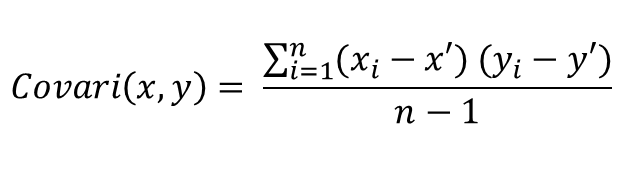
Here is the mathy-representation of the function we just implemented. This is the definition
of covariance.
That "S" symbol means summation and "i=1" means start at i=1 and go up to "n". This is the
mathy-way of saying loop through both arrays. Xi here represents a particular instance of x as we loop through our
arrays, and likewise Yi here represents a particular instance of y. X' and Y' represent the mean of our x and y
arrays, respectively.
So this formula is saying loop through each pair of points for x, and y and for each pair of
points, subtract the mean of the x array from x, and subtract the mean of the y array from y. Then take those two
values, and multiply them together and set them to the side. At the end sum all of these values up and divide the
value we get back by the length of the sample minus 1.
The function we wrote above is the Python/Numpy representation of this function. We used a
numpy array instead of a Python list as numpy allows us to do stuff like this really easily. When we write the
following line in numpy:
x - np.mean(x)
Numpy knows to return an array where each value in the original value had it's value reduced
by the mean of the original array. If we had used a Python list here, things would have been a bit more complicated.
By using the values attribute of our DataFrame column, we can get back the numpy
array representation of our column. The function we defined above only works with numpy arrays. We set x = usage and
y = FantasyPoints just as we did last time when we built the scatter plot.
What the hell does 8788 mean? I have no idea, and neither should you. This is why we
normalize our covariance because on it's own it's not super useful.
Luckily, the function for correlation is easier than the one for covariance.
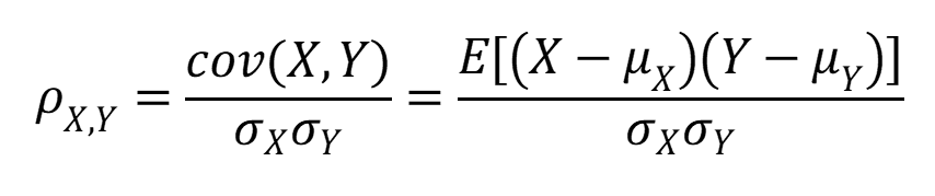
We just need that first part.
The correlation between two variables is their covariance divided by the product of their
standard deviations. We haven't gone over standard deviation, but we will eventually (it's pretty important for
analyzing picks in Fantasy Football). So we'll just be using a built-in function from our friend numpy
to write a very simple function.
Numpy has a built-in function called std which will calculate the standard
deviation of an array for us (It also has a cov function that calculates the covariance between two
arrays that I kept from you guys) and so our corr function we write here is pretty simple. We use our
function covariance we wrote earlier and then divide it by the product of the two standard deviations
of the arrays.
Conclusion
This was a long post, but was necessary as all of this stuff is laying the foundation for
building a linear regression model that will allow us to use usage to predict fantasy points. As you can see the
correlation between usage and fantasy points is about 0.97 for this sample, which is really high, so we'll move
forward with building a linear regression model.
I encourage you to alter our DataFrame we used for the x and y inputs and try to see the
correlation coefficients for usage v fantasy points for WR, TE, and QB. You'll have to adjust our definition of
usage for QB's (Add passing attempts, maybe).
Also, we used numpy's built-in std function here but you could have hard coded
this yourself and it's usually best when you're first learning this stuff to do so as it gives you a deeper
understanding of these basic statistic concepts. Try to look up the definition of standard deviation and maybe alter
the code to implement the function yourself (Without numpy).
 Photo by Evan Habeeb, USA TODAY Sports