If you have any questions about the code here, feel free to reach out to me on Twitter or on Reddit.
If you have any questions about the code here, feel free to reach out to me on Twitter or on Reddit.
Build an NFL Game Outcome and Win Probability Model in Python
This post was originally written for Open Source Football here, and has been adapted to the Fantasy Football Data Pros blog to share with my readers.
In this post we are going to cover predicting NFL game outcomes and pre-game win probability using a logistic regression model in Python. And since it's almost Super Bowl Sunday, at the end of the post we will be using the model to come up with a super bowl prediction!
Previous posts on Open Source Football have covered engineering EPA to maximize it's predictive value, and this post will partly build upon those written by Jack Lichtenstien and John Goldberg.
The goal of this post will be to provide you with an introduction to modeling in Python and a baseline model to work from. Python's de-facto machine learning library, sklearn, is built upon a streamlined API which allows ML code to be iterated upon easily. To switch to a more complex model wouldn't take much tweaking of the code I'll provide here, as every supervised algorithm is implemented via sklearn in more or less the same fashion.
As with any machine learning task, the bulk of the work will be in the data munging, cleaning, and feature extraction/engineering process.
For our features, we will be using exponentially weighted rolling EPA. For those who don't know what EPA is - it stands for estimated points added, and is a statistic that quantifies how many points a particular play added to a team's score. It's based on a lot of things - field position, yards gained, down and distance, etc. and is generally a good way to quantify and measure offensive and defensive efficiency/performance. A 30 yard play on 3rd and 13, for example, might have 3.2 estimated points added.
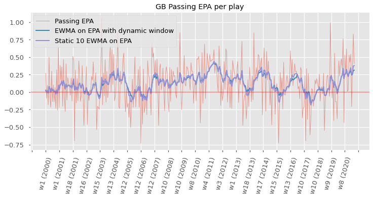
We will be taking average EPA per play for each team (split in to rushing, passing, and then further split in to defense, offense) for each week and then calculating a moving average (we will also lag the data back one period, so we only use data up to and not including a particular game). Moreover, instead of calculating a simple moving average, we will be calculating a exponential moving average, which will weigh more recent games more heavily.
The window size for the rolling average will be 10 for all teams before week 10 of the season. This means that prior to week 10, some prior season data will be used. If we're past week 10, the entire, and only the entire, season will be included in the calculation of rolling EPA. This dynamic window size idea was Jack Lichtenstien's, and his post on Open Source Football on the topic is linked above. His post showed that using a dynamic window size was slightly more predictive than using a static 10 game window.
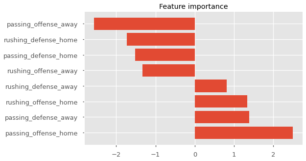
EPA will be split in to defense and offense for both teams, and then further split in to passing and rushing. This means in total, we'll have 8 features:
1. Home team passing offense EPA/play
2. Home team passing defense EPA/play
3. Home team rushing offense EPA/play
4. Home team rushing defense EPA/play
5. Away team passing offense EPA/play
6. Away team passing defense EPA/play
7. Away team rushing offense EPA/play
8. Away team rushing defense EPA/play
The target will be a home team win.
Each of these features will be lagged one period, and then an exponential moving average will be calculated.
We're going to be using Logistic Regression as our model. Logistic Regression is used to model the probability of a binary outcome. The probability we are attempting to model here is the probability a home team wins given the features we've laid out above. We'll see that our LogisticRegression object has a predict_proba method which shows us the predicted probability of a 1 (home team win) or 0 (away team win). This means the model can be used as a pre-game win probability model as well.
We'll be training the model with data from 1999 - 2019, and leaving 2020 out so we can analyze it further at the end of the post.
To start, let's install the nflfastpy module, a Python package I manage which allows us easy access to nflfastR data.
Next, we import some stuff we'll need for this notebook and also set the base styling for our matplotlib visualizations.
The code block below will pull nflfastR data from the [nflfastR-data](https://github.com/guga31bb/nflfastR-data) repository and concatenate the seperate, yearly DataFrames in to a single DataFrame we'll call data. This code block will take anywhere from 2-5 minutes.
The code below is going to calculate a rolling EPA with a static window and a dynamic window. I've included both, although we'll only be using the rolling EPA with the dynamic window in our model.
|
team |
season |
week |
epa_rushing_offense |
epa_shifted_rushing_offense |
ewma_rushing_offense |
ewma_dynamic_window_rushing_offense |
epa_passing_offense |
epa_shifted_passing_offense |
ewma_passing_offense |
ewma_dynamic_window_passing_offense |
epa_rushing_defense |
epa_shifted_rushing_defense |
ewma_rushing_defense |
ewma_dynamic_window_rushing_defense |
epa_passing_defense |
epa_shifted_passing_defense |
ewma_passing_defense |
ewma_dynamic_window_passing_defense |
| 0 |
ARI |
2000 |
1 |
-0.345669 |
-0.068545 |
-0.109256 |
-0.109256 |
0.018334 |
0.056256 |
-0.172588 |
-0.172588 |
0.202914 |
0.363190 |
0.080784 |
0.080784 |
-0.069413 |
0.269840 |
0.119870 |
0.119870 |
| 1 |
ARI |
2000 |
2 |
-0.298172 |
-0.345669 |
-0.153707 |
-0.153707 |
0.587000 |
0.018334 |
-0.136691 |
-0.136691 |
-0.110405 |
0.202914 |
0.103747 |
0.103747 |
0.311383 |
-0.069413 |
0.084280 |
0.084280 |
| 2 |
ARI |
2000 |
4 |
-0.334533 |
-0.298172 |
-0.180702 |
-0.180702 |
-0.271663 |
0.587000 |
-0.001460 |
-0.001460 |
-0.018524 |
-0.110405 |
0.063730 |
0.063730 |
0.500345 |
0.311383 |
0.126717 |
0.126717 |
| 3 |
ARI |
2000 |
5 |
-0.041279 |
-0.334533 |
-0.209303 |
-0.209303 |
0.069246 |
-0.271663 |
-0.051697 |
-0.051697 |
0.012054 |
-0.018524 |
0.048437 |
0.048437 |
0.058499 |
0.500345 |
0.196184 |
0.196184 |
| 4 |
ARI |
2000 |
6 |
-0.038473 |
-0.041279 |
-0.178191 |
-0.178191 |
0.101830 |
0.069246 |
-0.029303 |
-0.029303 |
0.086308 |
0.012054 |
0.041700 |
0.041700 |
-0.063633 |
0.058499 |
0.170690 |
0.170690 |
We can plot EPA for the Green Bay Packers alongside our moving averages. We can see that the static window EMA and dynamic window EMA are quite similar, with slight divergences towards season ends.
Now that we have our features compiled, we can begin to merge in game result data to come up with our target variable.
|
season |
week |
home_team |
away_team |
home_score |
away_score |
home_team_win |
epa_rushing_offense_home |
epa_shifted_rushing_offense_home |
ewma_rushing_offense_home |
... |
ewma_passing_offense_away |
ewma_dynamic_window_passing_offense_away |
epa_rushing_defense_away |
epa_shifted_rushing_defense_away |
ewma_rushing_defense_away |
ewma_dynamic_window_rushing_defense_away |
epa_passing_defense_away |
epa_shifted_passing_defense_away |
ewma_passing_defense_away |
ewma_dynamic_window_passing_defense_away |
| 0 |
2000 |
1 |
NYG |
ARI |
21 |
16 |
1 |
0.202914 |
0.162852 |
-0.108683 |
... |
-0.172588 |
-0.172588 |
0.202914 |
0.363190 |
0.080784 |
0.080784 |
-0.069413 |
0.269840 |
0.119870 |
0.119870 |
| 1 |
2000 |
1 |
PIT |
BAL |
0 |
16 |
0 |
-0.499352 |
-0.643877 |
-0.128608 |
... |
-0.115204 |
-0.115204 |
-0.499352 |
-0.241927 |
-0.167554 |
-0.167554 |
-0.216112 |
-0.208568 |
-0.197401 |
-0.197401 |
| 2 |
2000 |
1 |
WAS |
CAR |
20 |
17 |
1 |
-0.006129 |
-0.498218 |
-0.076112 |
... |
0.227056 |
0.227056 |
-0.006129 |
0.060270 |
0.064942 |
0.064942 |
0.147979 |
-0.368611 |
0.001883 |
0.001883 |
| 3 |
2000 |
1 |
MIN |
CHI |
30 |
27 |
1 |
0.283000 |
-0.115150 |
-0.058772 |
... |
-0.079775 |
-0.079775 |
0.283000 |
-0.130394 |
-0.045563 |
-0.045563 |
0.124496 |
0.365886 |
0.106074 |
0.106074 |
| 4 |
2000 |
1 |
LA |
DEN |
41 |
36 |
1 |
-0.106372 |
-0.692095 |
-0.263223 |
... |
-0.011590 |
-0.011590 |
-0.106372 |
-0.110182 |
-0.063446 |
-0.063446 |
0.400226 |
-0.078273 |
-0.089393 |
-0.089393 |
5 rows × 39 columns
We'll set some variables to isolate our target and features. Here, we are only including the dynamic window columns. I've found that the dynamic window does produce a slightly better model score. You're welcome to use the EWMA features with the static window size.
Here, we finally train and test our model. In sklearn, each supervised algorithm is implemented in the same fashion, First, you bring in your class (which we did earlier in the code). You then instantiate the class, providing model hyperparameters at instantiation. Here, since we're just doing Logistic Regression, we have none (although sklearn allows us to provide C as a hyperpameter - which controls regularization). Then, you call the fit method which trains your model. For evaluating model accuracy, you have a couple options. Notice here we did not split our model in to train and test sets, as we'll be using 10-fold cross validation to train and test instead using the cross_val_scores function we brought in earlier.
We see our week model has about a 63.5% accuracy score. Not terrible, considering if you head over to nflpickwatch.com, you'll see that the best experts tend to cluster around 68%.
We also found the negative log loss. This is important because the model could have value as a win probability model as opposed to a straight pick-em model.
The model can definitely be improved. Some possible improvements and things I'd like to explore in future iterations of this model:
1. Using John Goldberg's idea of opponent-adjusted EPA
2. Weighing EPA by win probability
3. Engineering other features beyond EPA, including special teams performance
4. Switch to a more complex model + hyperparameter tuning
Something fun we can do now is see how the model would have predicted this past season. Notice we took out 2020 data from our training data, and so now we are free to see how the model would have done in 2020 (since none of the 2020 data was used for training).
|
home_team |
away_team |
week |
predicted_winner |
actual_winner |
win_probability |
correct_prediction |
| 0 |
KC |
NYJ |
8 |
KC |
KC |
0.874193 |
1 |
| 1 |
KC |
DEN |
13 |
KC |
KC |
0.845162 |
1 |
| 2 |
LA |
NYJ |
15 |
LA |
NYJ |
0.833220 |
0 |
| 3 |
LA |
NYG |
4 |
LA |
LA |
0.832061 |
1 |
| 4 |
SF |
PHI |
4 |
SF |
PHI |
0.819993 |
0 |
| 5 |
MIA |
NYJ |
6 |
MIA |
MIA |
0.802636 |
1 |
| 6 |
BAL |
CLE |
1 |
BAL |
BAL |
0.794298 |
1 |
| 7 |
KC |
CAR |
9 |
KC |
KC |
0.793608 |
1 |
| 8 |
BAL |
CIN |
5 |
BAL |
BAL |
0.779855 |
1 |
| 9 |
IND |
JAX |
17 |
IND |
IND |
0.773426 |
1 |
These are the 10 games this season the model was most confident about. No surprises here that the KC-NYJ game was the most lopsided game this season.
We can also view how our model would have done this season by week. There doesn't seem to be a clear trend here. You would expect that the model would get better as the season went on, but the data doesn't make that clear here.
The model would have done the best in week 2 of the 2020 season, with a 87.5% accuracy score!
|
home_team |
away_team |
week |
predicted_winner |
actual_winner |
win_probability |
correct_prediction |
| 5341 |
TB |
CAR |
2 |
TB |
TB |
0.763676 |
1 |
| 5339 |
HOU |
BAL |
2 |
BAL |
BAL |
0.743131 |
1 |
| 5345 |
TEN |
JAX |
2 |
TEN |
TEN |
0.740741 |
1 |
| 5344 |
GB |
DET |
2 |
GB |
GB |
0.733028 |
1 |
| 5353 |
ARI |
WAS |
2 |
ARI |
ARI |
0.708931 |
1 |
| 5338 |
DAL |
ATL |
2 |
DAL |
DAL |
0.694735 |
1 |
| 5351 |
CHI |
NYG |
2 |
CHI |
CHI |
0.645196 |
1 |
| 5343 |
PIT |
DEN |
2 |
PIT |
PIT |
0.640730 |
1 |
| 5349 |
SEA |
NE |
2 |
SEA |
SEA |
0.636207 |
1 |
| 5346 |
LAC |
KC |
2 |
KC |
KC |
0.596137 |
1 |
| 5342 |
CLE |
CIN |
2 |
CLE |
CLE |
0.556421 |
1 |
| 5340 |
MIA |
BUF |
2 |
BUF |
BUF |
0.556119 |
1 |
| 5352 |
NYJ |
SF |
2 |
SF |
SF |
0.553112 |
1 |
| 5350 |
LV |
NO |
2 |
NO |
LV |
0.532511 |
0 |
| 5348 |
IND |
MIN |
2 |
IND |
IND |
0.520469 |
1 |
| 5347 |
PHI |
LA |
2 |
PHI |
LA |
0.515421 |
0 |
We can also view how our model would have done in the playoffs by filtering out weeks prior to week 17.
|
home_team |
away_team |
week |
predicted_winner |
actual_winner |
win_probability |
correct_prediction |
| 5578 |
TEN |
BAL |
18 |
BAL |
BAL |
0.551507 |
1 |
| 5579 |
NO |
CHI |
18 |
NO |
NO |
0.755613 |
1 |
| 5580 |
PIT |
CLE |
18 |
PIT |
CLE |
0.513341 |
0 |
| 5581 |
BUF |
IND |
18 |
BUF |
BUF |
0.632864 |
1 |
| 5582 |
SEA |
LA |
18 |
SEA |
LA |
0.589866 |
0 |
| 5583 |
WAS |
TB |
18 |
TB |
TB |
0.614521 |
1 |
| 5584 |
BUF |
BAL |
19 |
BUF |
BUF |
0.527067 |
1 |
| 5585 |
KC |
CLE |
19 |
KC |
KC |
0.587855 |
1 |
| 5586 |
GB |
LA |
19 |
GB |
GB |
0.689657 |
1 |
| 5587 |
NO |
TB |
19 |
NO |
TB |
0.597603 |
0 |
| 5588 |
KC |
BUF |
20 |
KC |
KC |
0.530803 |
1 |
| 5589 |
GB |
TB |
20 |
GB |
TB |
0.593343 |
0 |
Of course, an NFL game prediction post a week out from the super bowl isn't complete without a super bowl prediction.
Final Thoughts
The goal of this post was to provide you with a baseline model to work from in Python that can be easily iterated upon.
The model was came out to be around 63.5% accurate, and can definitely be improved on. The model may also have more value as a pre-game win probability model.
In future posts, I would like to incorporate EPA adjusted for opponent and also look at how WP affects the predictability of EPA, as it's an interesting idea and I think there could be some value there. Also, trying out other features besides EPA could certainly help. Turnover rates, time of possession, average number of plays ran, average starting field position, special teams performance, QB specific play, etc, could all prove useful. We saw in the visualization of feature importance that passing EPA per play had the most predictive power for a home team win and away team win. Exploring QB specific features could help improve the model. Of course, that would require roster data for each week.
As always - thank you for reading!
 Photo by David Eulitt, Getty Images