Learn Python with Fantasy Football: Which receivers are under performing their season?

Use a linear regression model with sklearn to find which players are under performing through 10 weeks.
Use a linear regression model with sklearn to find which players are under performing through 10 weeks.
If you have any questions about the code here, feel free to reach out to me on Twitter or on Reddit.
In this part of the Learn Python with Fantasy Football season, we're going to use a linear regression model to find who is "underperforming" their season given their air yards and also number of targets.
This is just going to be a fun implementation of regression to find those players who are not performing where they should be given a line of best fit on the data. Air yards and targets are somewhat predictive of fantasy football performance, but there's obviously much more to it than that. The players who are exceptionally good at creating yards after catch will outperform any model based on averages. Kamara has barely seen any air yards all season, yet he'd still be a top fantasy player if you only counted his fantasy points as a result of his receiving yards, catches, and receiving TDs.
To start off, we'll create some simple scatter plots to visualize the relationship between targets and air yards and fantasy football performance. Then, we'll move on to implementing the model, and then analyzing the residuals. Those players with a large negative residual between expected fantasy points and actual fantasy points are said to be due for some positive regression. I'm writing this post as I'm writing the code, so I have no idea what to expect. Apologies now if the results are wacky. I have a feeling Marquez-Valdez Scantling is going to show up as an underperformer, but if you start him next week based on this post and he drops a dougnut, please don't email me.
Let's start off with installing the nflfastpy library in to your Google Colab notebook.
Aaand importing our libraries as always. Some new ones here from sklearn. We are importing the LinearRegression class to actually implement our model, and the mean_absolute_error utility function to evaluate our results.
Let's load 2019 and 2020 data. We're going to be using 2019 data to train our model, and 2020 data to predict values.
Before we move on, the data loading process takes a few moments, so let's make some copies of our data so we don't have to run the cell block above again.
Now, let's write a function that's going to aggregate the data we need from the play by play data.
| receiver_player_id | receiver_player_name | game_id | targets | catches | air_yards | yards_gained | rec_td | rec_fpts | |
|---|---|---|---|---|---|---|---|---|---|
| 0 | 32013030-2d30-3032-3231-32373ce51f62 | J.Witten | 2019_01_NYG_DAL | 4.0 | 3.0 | 3.0 | 15.0 | 1.0 | 10.5 |
| 1 | 32013030-2d30-3032-3231-32373ce51f62 | J.Witten | 2019_02_DAL_WAS | 4.0 | 4.0 | 15.0 | 25.0 | 1.0 | 12.5 |
| 2 | 32013030-2d30-3032-3231-32373ce51f62 | J.Witten | 2019_03_MIA_DAL | 4.0 | 3.0 | 42.0 | 54.0 | 0.0 | 8.4 |
| 3 | 32013030-2d30-3032-3231-32373ce51f62 | J.Witten | 2019_04_DAL_NO | 4.0 | 4.0 | 40.0 | 50.0 | 0.0 | 9.0 |
| 4 | 32013030-2d30-3032-3231-32373ce51f62 | J.Witten | 2019_05_GB_DAL | 4.0 | 3.0 | 57.0 | 29.0 | 0.0 | 5.9 |
We now have weekly data available for 2019. Let's visualize the relationship between air yards and receiving fantasy points.
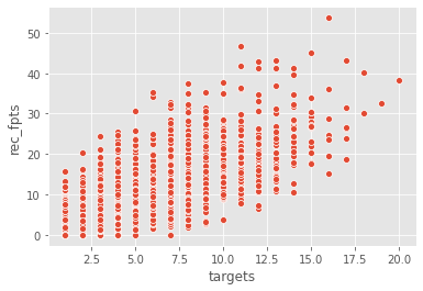
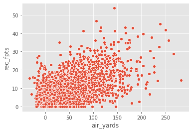
We can see there is some sort of relationship between air yards/targets and receiving fantasy points output.
Let's move on to implementing a model based on these relationship for fantasy points scored.
First, we are going to split up our features (X) and target (y). Our features are what we are using to predict fantasy points, air yards and targets, and our target is fantasy points.
We are also going to double check and make sure we don't have any null values in our Data, which we probably don't.
Now that we know we have no null values, let's covert these DataFrames to numpy arrays using the values attribute.
Our model can be implemented as simply as the one-liner below.
Now that we have a model fitted on 2019 data, let's use it to predict 2020 numbers (that already happened). Again, the point here is not to predict future performance, that would require us to know how many targets and air yards a player will have next week in advance. The point here is to ensure we have a decent model, use it to predict past values, and then see which players are underperforming or overperforming based on the expected model.
| receiver_player_id | receiver_player_name | game_id | targets | catches | air_yards | yards_gained | rec_td | rec_fpts | rec_fpts_pred | |
|---|---|---|---|---|---|---|---|---|---|---|
| 0 | 32013030-2d30-3032-3231-32373ce51f62 | J.Witten | 2020_01_LV_CAR | 1.0 | 1.0 | 2.0 | 2.0 | 0.0 | 1.2 | 1.589535 |
| 1 | 32013030-2d30-3032-3231-32373ce51f62 | J.Witten | 2020_02_NO_LV | 1.0 | 1.0 | 3.0 | 3.0 | 0.0 | 1.3 | 1.608743 |
| 2 | 32013030-2d30-3032-3231-32373ce51f62 | J.Witten | 2020_04_BUF_LV | 2.0 | 2.0 | 18.0 | 18.0 | 1.0 | 9.8 | 3.426626 |
| 3 | 32013030-2d30-3032-3231-32373ce51f62 | J.Witten | 2020_05_LV_KC | 2.0 | 2.0 | -1.0 | 6.0 | 0.0 | 2.6 | 3.061687 |
| 4 | 32013030-2d30-3032-3231-32373ce51f62 | J.Witten | 2020_07_TB_LV | 1.0 | 1.0 | 3.0 | 6.0 | 0.0 | 1.6 | 1.608743 |
Let's see how good our model was at predicting 2020 values.
Our model was off by about 3 fantasy points per game. This means most of our predictions were +- within 3 of the actual results.
We're going to create a new column now to calculate the difference between y_true and y_pred (our residual).
| receiver_player_id | receiver_player_name | game_id | targets | catches | air_yards | yards_gained | rec_td | rec_fpts | rec_fpts_pred | residual | |
|---|---|---|---|---|---|---|---|---|---|---|---|
| 0 | 32013030-2d30-3032-3231-32373ce51f62 | J.Witten | 2020_01_LV_CAR | 1.0 | 1.0 | 2.0 | 2.0 | 0.0 | 1.2 | 1.589535 | -0.389535 |
| 1 | 32013030-2d30-3032-3231-32373ce51f62 | J.Witten | 2020_02_NO_LV | 1.0 | 1.0 | 3.0 | 3.0 | 0.0 | 1.3 | 1.608743 | -0.308743 |
| 2 | 32013030-2d30-3032-3231-32373ce51f62 | J.Witten | 2020_04_BUF_LV | 2.0 | 2.0 | 18.0 | 18.0 | 1.0 | 9.8 | 3.426626 | 6.373374 |
| 3 | 32013030-2d30-3032-3231-32373ce51f62 | J.Witten | 2020_05_LV_KC | 2.0 | 2.0 | -1.0 | 6.0 | 0.0 | 2.6 | 3.061687 | -0.461687 |
| 4 | 32013030-2d30-3032-3231-32373ce51f62 | J.Witten | 2020_07_TB_LV | 1.0 | 1.0 | 3.0 | 6.0 | 0.0 | 1.6 | 1.608743 | -0.008743 |
Let's sort values by the residual column to see when our model was most wrong.
| receiver_player_id | receiver_player_name | game_id | targets | catches | air_yards | yards_gained | rec_td | rec_fpts | rec_fpts_pred | residual | |
|---|---|---|---|---|---|---|---|---|---|---|---|
| 1188 | 32013030-2d30-3033-3337-353731d69d3c | R.Tonyan | 2020_04_ATL_GB | 6.0 | 6.0 | 63.0 | 98.0 | 3.0 | 33.8 | 10.410052 | 23.389948 |
| 910 | 32013030-2d30-3033-3331-3130f1a1e2e4 | T.Higbee | 2020_02_LA_PHI | 5.0 | 5.0 | 44.0 | 54.0 | 3.0 | 28.4 | 8.515338 | 19.884662 |
| 2307 | 32013030-2d30-3033-3633-32324e92bd12 | J.Jefferson | 2020_06_ATL_MIN | 11.0 | 9.0 | 137.0 | 166.0 | 2.0 | 37.6 | 19.480263 | 18.119737 |
| 716 | 32013030-2d30-3033-3232-31312f766863 | T.Lockett | 2020_07_SEA_ARI | 20.0 | 15.0 | 233.0 | 200.0 | 3.0 | 53.0 | 35.092131 | 17.907869 |
| 1284 | 32013030-2d30-3033-3339-3036f296898c | A.Kamara | 2020_03_GB_NO | 14.0 | 13.0 | -8.0 | 139.0 | 2.0 | 38.9 | 21.284519 | 17.615481 |
The first result makes sense, Robert Tonyan scored a TD on half of his targets. It looks like our model is pretty bad at predicting multiple TD games. Let's use a simple scatter plot to analyze further.
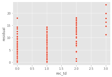
Yup, so our model got progressively worse the more a player scored a TD in a given game. 0 and 1 TD games it was alright, but 3 TD games it could not handle.
Let's move on to joining some injury data to remove injured players and then finding some underperformers anyhow.
There's a new function in the nflfastpy module that let's you load 2020 roster data. It contains data on injured players too which is pretty neat.
| season | team | position | depth_chart_position | jersey_number | status | full_name | first_name | last_name | birth_date | ... | weight | college | high_school | gsis_id | espn_id | sportradar_id | yahoo_id | rotowire_id | update_dt | headshot_url | |
|---|---|---|---|---|---|---|---|---|---|---|---|---|---|---|---|---|---|---|---|---|---|
| 0 | 2020 | ARI | C | C | 52.0 | Active | Mason Cole | Mason | Cole | 1996-03-28 | ... | 292.0 | Michigan | East Lake (FL) | 00-0034785 | 3115972.0 | 53d25371-e3ce-4030-8d0a-82def5cdc600 | 31067.0 | 12795.0 | 2020-11-21T07:08:46Z | https://a.espncdn.com/combiner/i?img=/i/headsh... |
1 rows × 21 columns
| receiver_player_id | receiver_player_name | game_id | targets | catches | air_yards | yards_gained | rec_td | rec_fpts | rec_fpts_pred | residual | gsis_id | status | headshot_url | |
|---|---|---|---|---|---|---|---|---|---|---|---|---|---|---|
| 0 | 32013030-2d30-3032-3231-32373ce51f62 | J.Witten | 2020_01_LV_CAR | 1.0 | 1.0 | 2.0 | 2.0 | 0.0 | 1.2 | 1.589535 | -0.389535 | 00-0022127 | Active | https://a.espncdn.com/combiner/i?img=/i/headsh... |
| 1 | 32013030-2d30-3032-3231-32373ce51f62 | J.Witten | 2020_02_NO_LV | 1.0 | 1.0 | 3.0 | 3.0 | 0.0 | 1.3 | 1.608743 | -0.308743 | 00-0022127 | Active | https://a.espncdn.com/combiner/i?img=/i/headsh... |
| 2 | 32013030-2d30-3032-3231-32373ce51f62 | J.Witten | 2020_04_BUF_LV | 2.0 | 2.0 | 18.0 | 18.0 | 1.0 | 9.8 | 3.426626 | 6.373374 | 00-0022127 | Active | https://a.espncdn.com/combiner/i?img=/i/headsh... |
| 3 | 32013030-2d30-3032-3231-32373ce51f62 | J.Witten | 2020_05_LV_KC | 2.0 | 2.0 | -1.0 | 6.0 | 0.0 | 2.6 | 3.061687 | -0.461687 | 00-0022127 | Active | https://a.espncdn.com/combiner/i?img=/i/headsh... |
| 4 | 32013030-2d30-3032-3231-32373ce51f62 | J.Witten | 2020_07_TB_LV | 1.0 | 1.0 | 3.0 | 6.0 | 0.0 | 1.6 | 1.608743 | -0.008743 | 00-0022127 | Active | https://a.espncdn.com/combiner/i?img=/i/headsh... |
Awesome, so we converted the receiver id to the old gsis id like we've done in previous posts, and then merged the roster data and filtered out inactive players. Let's move on to filtering out some unneccesary columns and preparing our data for more analysis.
| gsis_id | receiver_player_name | headshot_url | rec_fpts | rec_fpts_pred | residual | |
|---|---|---|---|---|---|---|
| 0 | 00-0022127 | J.Witten | https://a.espncdn.com/combiner/i?img=/i/headsh... | 1.2 | 1.589535 | -0.389535 |
| 1 | 00-0022127 | J.Witten | https://a.espncdn.com/combiner/i?img=/i/headsh... | 1.3 | 1.608743 | -0.308743 |
| 2 | 00-0022127 | J.Witten | https://a.espncdn.com/combiner/i?img=/i/headsh... | 9.8 | 3.426626 | 6.373374 |
| 3 | 00-0022127 | J.Witten | https://a.espncdn.com/combiner/i?img=/i/headsh... | 2.6 | 3.061687 | -0.461687 |
| 4 | 00-0022127 | J.Witten | https://a.espncdn.com/combiner/i?img=/i/headsh... | 1.6 | 1.608743 | -0.008743 |
Let's group by receiver and find the players who our model favored the most.
| gsis_id | receiver_player_name | headshot_url | rec_fpts | rec_fpts_pred | residual | |
|---|---|---|---|---|---|---|
| 72 | 00-0031381 | D.Adams | https://a.espncdn.com/combiner/i?img=/i/headsh... | 27.014286 | 19.745273 | 7.269013 |
| 83 | 00-0031588 | S.Diggs | https://a.espncdn.com/combiner/i?img=/i/headsh... | 18.760000 | 17.436972 | 1.323028 |
| 44 | 00-0030279 | K.Allen | https://a.espncdn.com/combiner/i?img=/i/headsh... | 18.222222 | 17.433888 | 0.788334 |
| 55 | 00-0030564 | D.Hopkins | https://a.espncdn.com/combiner/i?img=/i/headsh... | 18.820000 | 16.508142 | 2.311858 |
| 325 | 00-0035659 | T.McLaurin | https://a.espncdn.com/combiner/i?img=/i/headsh... | 17.077778 | 16.440406 | 0.637372 |
Adams, Diggs, Allen, Hopkins, and McLaurin are our models top expected receivers for this year. We can see that Adams has a large average residual, probably as a result of his TD production.
We can also see that our model is really conservative. Let's get rid of the predicted values and just use a rank instead.
| receiver_player_name | headshot_url | rec_fpts | rec_fpts_pred | residual | |
|---|---|---|---|---|---|
| 72 | D.Adams | https://a.espncdn.com/combiner/i?img=/i/headsh... | 1.0 | 1.0 | 7.269013 |
| 83 | S.Diggs | https://a.espncdn.com/combiner/i?img=/i/headsh... | 7.0 | 2.0 | 1.323028 |
| 44 | K.Allen | https://a.espncdn.com/combiner/i?img=/i/headsh... | 8.0 | 3.0 | 0.788334 |
| 55 | D.Hopkins | https://a.espncdn.com/combiner/i?img=/i/headsh... | 5.5 | 4.0 | 2.311858 |
| 325 | T.McLaurin | https://a.espncdn.com/combiner/i?img=/i/headsh... | 15.0 | 5.0 | 0.637372 |
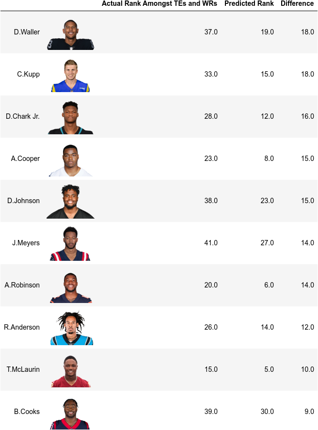
So now we have expected rank and also actual rank. Finally, let's find the biggest differences between expected rank and actual rank
| receiver_player_name | headshot_url | rec_fpts | rec_fpts_pred | diff | |
|---|---|---|---|---|---|
| 85 | D.Waller | https://a.espncdn.com/combiner/i?img=/i/headsh... | 37.0 | 19.0 | 18.0 |
| 191 | C.Kupp | https://a.espncdn.com/combiner/i?img=/i/headsh... | 33.0 | 15.0 | 18.0 |
| 265 | D.Chark Jr. | https://a.espncdn.com/combiner/i?img=/i/headsh... | 28.0 | 12.0 | 16.0 |
| 79 | A.Cooper | https://a.espncdn.com/combiner/i?img=/i/headsh... | 23.0 | 8.0 | 15.0 |
| 294 | D.Johnson | https://a.espncdn.com/combiner/i?img=/i/headsh... | 38.0 | 23.0 | 15.0 |
Darren Waller is our biggest underperformer for the 2020 season so far. He should be ranked 19 amongst all WRs and TEs, but he's only ranked 37.
Let's style our DataFrame and call it a day.