If you have any questions about the code here, feel free to reach out to me on Twitter or on Reddit.
Shameless Plug Section
If you like Fantasy Football and have an interest in learning how to code, check out our
Ultimate Guide on Learning Python with Fantasy Football Online Course. Here is a link to purchase for
15% off. The course includes 15 chapters of material, 14 hours of video, hundreds of data sets, lifetime
updates, and a Slack channel invite to join the Fantasy Football with Python community.
Introductions and Humble Brags
In this post we are going to be begin a series on using the programming language Python for
fantasy football data analysis. Over the past season, I started using Python to make decisions on who to start
every week, and maybe it’s just a coincidence – but I finally won the ‘ship this year (insert humble brag).
I believe Python can be an incredible tool for making fantasy football decisions, but there
is little information on the internet on how to actually get started. This post is going to be about setting up
a Python environment with anaconda, jupyter, pandas,
seaborn, and matplotlib, and then at the end we will do some basic analysis of
efficiency versus usage for running backs.
Getting Python Set Up
To start, you are going to need Anaconda, which is essentially a distribution of Python
made for data science. You
can find a link to the download section here.
Easily enough, anaconda already comes with almost everything we need to get started
(Including jupyter, numpy, pandas, seaborn, and matplotlib). Anaconda also comes with it’s own terminal, which
we’ll be using for the remainder of the series. Fire up the Anaconda Prompt after you’re done installing, and
make a new directory for your jupyter notebooks (More on this in a bit).
mkdir fantasyfootball
cd fantasyfootball
We’re going to be doing almost all our Python in Jupyter notebooks. For those unfamiliar
with Jupyter notebooks, they are essentially a web based interface where you can write Python code in “cells”.
They’re really useful for exploratory hacking, and you’ll see why in a minute. In your directory, type the
following command to open a new instance of Jupyter.
You should see that Jupyter is now running on your localhost. If it hasn’t already automatically
popped up for you, type into your browser localhost:[whatever port your terminal says]/tree. Once
you’re there, click on the “new” dropdown on the right hand side, and from the dropdown select to create a new
Python3 notebook.
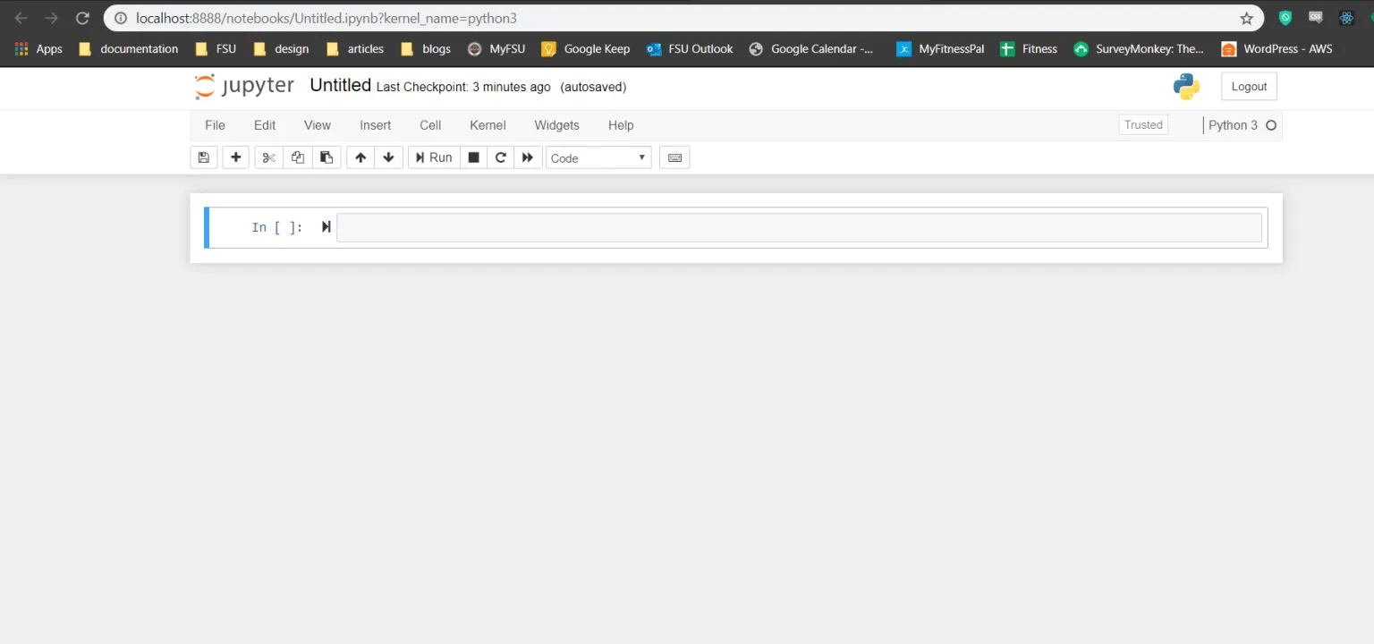
You should see this in your browser. Change the name from “Untitled” to whatever you want.
I named mine the name of this post but it doesn’t really matter.
Our Dataset
We are almost done with the setup before we start coding. The last thing we need to do is
get a dataset. I was able to easily grab data sets from profootballreference.com for free, however, you’re free
to use whatever source you want, as long as the file is in CSV/Excel format. For this part, we are going to be
using a 2019 dataset consisting of every WR, RB, TE, and QB that played this year. Later, we will filter and
separate this dataset into four different data sets based on position using the Python library pandas. I’ve
included the CSV file taken from profootball reference. Download and place the file within your project
directory (This is important. If it’s not in the same directory as your jupyter notebooks we won’t be able to
read it). Save the file as 2019.csv
Our First Lines of Code
Finally, we can begin coding. Again, for those unfamiliar with Jupyter notebooks, we are
writing python code within these “cells” and then running these cells using Shift+Enter. You can
write multiple lines of code within each cell, and it’s probably better that you do. Just separate each cell
based off function or purpose much like you would any other .py file. For more information on jupyter, check out
the docs here https://jupyter.org/documentation.
We’ll begin by importing some of the libraries we are going to be using.
import pandas as pd
import seaborn as sns
from matplotlib import pyplot as plt
Briefly, pandas is a python library included in anaconda which allows us to work with
“DataFrames”. DataFrames are like Excel spreadsheets that can be manipulated using pandas. Pandas will be the
most important and powerful library we will use and probably provide the steepest learning curve. For the
purposes of this post, we won’t be going over all the basics of pandas as that would necessitate an entire post.
I advise you check out the pandas documentation here https://pandas.pydata.org/pandas-docs/stable/ .
Matplotlib and seaborn are both used for data visualization and plotting, and the basics can be learned fairly
quickly. Run this cell using Shift+Enter and ensure there are no import errors (There shouldn’t
be).
Next, we are going to import our CSV file and create a pandas DataFrame, clean up the data, and then
separate the DataFrame into four different DataFrames for each position being analyzed – RB, WR, QB, and TE.
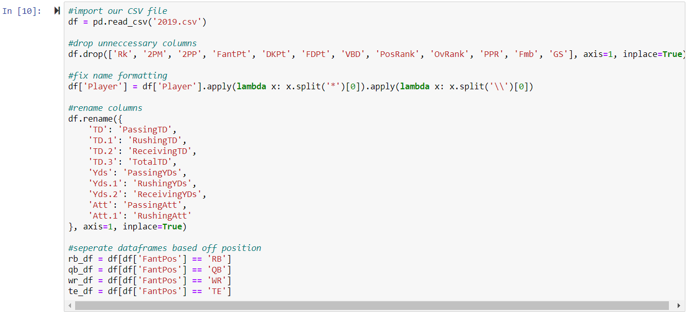
Our First Block of Code (After Importing)
This is a lot to unpack, so let’s take it step by step.
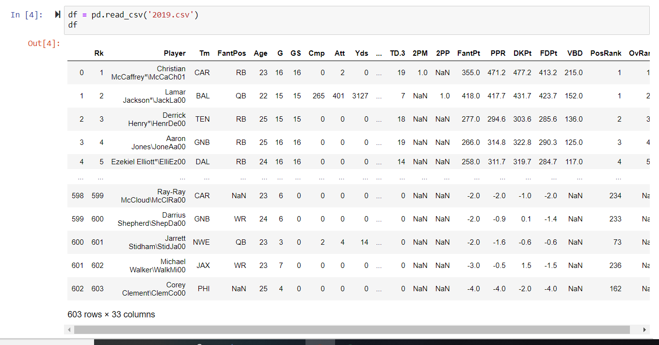
On the first line, we use the function from pandas called read_csv to read our CSV file
and convert it to a DataFrame. If you type in df on the next line and run the cell, you can actually see our
DataFrame.
You’ll probably notice some issues with our DataFrame right away. First of all, the
formatting for the player names is all messed up. Second of all, there’s a lot of unnecessary columns that
probably won’t be necessary for the purposes of our analysis. Third of all, we have repeating values (eg. TD,
TD.1, TD.2, TD.3).
df.drop(['Rk', '2PM', '2PP', 'FantPt', 'DKPt', 'FDPt', 'VBD', 'PosRank', 'OvRank', 'PPR', 'Fmb', 'GS'], axis=1, inplace=True)
To drop columns from a pandas DataFrame, you simple use the .drop built-in method for the
DataFrame, pass in a list of column names, set axis = 1, and set inplace = True.
Setting axis = 1 tells pandas that we are committing a change on the column axis. In pandas, 0 is
the row axis and 1 is the column axis. Setting inplace=True tells pandas to make a permanent change
to our DataFrame.
By the way, if you want to see your DataFrame but don’t want to produce the entire table,
use the built-in methods .head() and .tail(). By default, .head()
produces a DataFrame with the top 5 rows (try to guess what .tail() does). You can pass in an
argument for the number of rows but the default is 5. For example, df.head(10) would produce the top 10 rows.
df['Player'] = df['Player'].apply(lambda x: x.split('*')[0]).apply(lambda x: x.split('\\')[0])
You edit columns in pandas using the syntax df[“Column Name”]. The apply
built-in method allows you to run a function across an entire column axis. I used a lambda function for
simplicity to clean up the player name column. You can chain functions to apply multiple functions at once.
Those unfamiliar with lambda functions can check out the documentation here. If you’ve ever coded in
JavaScript, lambda functions are very similar to arrow functions.
df.rename({
'TD': 'PassingTD',
'TD.1': 'RushingTD',
'TD.2': 'ReceivingTD',
'TD.3': 'TotalTD',
'Yds': 'PassingYDs',
'Yds.1': 'RushingYDs',
'Yds.2': 'ReceivingYDs',
'Att': 'PassingAtt',
'Att.1': 'RushingAtt'
}, axis=1, inplace=True)
Another built-in method for pandas DataFrames is rename, which allows you to rename column
names. Again, we use axis=1 to indicate that we are making a change on the column axis, and we set
inplace=True to tell pandas that we want to make a permanent change to our DataFrame.
#separate dataframes based off position
rb_df = df[df['FantPos'] == 'RB']
qb_df = df[df['FantPos'] == 'QB']
wr_df = df[df['FantPos'] == 'WR']
te_df = df[df['FantPos'] == 'TE']
Here, we are creating four different DataFrames based off the column row ‘FantPos’. For
rb_df, for example, we are saying to pandas create a new DataFrame where ‘FantPos’ =
‘RB’. The syntax for how this is done is df[df[“Column Name”] == “Some Value”]]. We can
also use our other operators besides ==, such as, >, <,
!=, etc. We will see this is extremely powerful and useful when we want some minimum criteria.
Later on, we will be evaluating the correlation between TD/Number of Carries (Efficiency) and Fantasy Points/GM.
Obviously, we want to eliminate those players with a small number of carries. For example, fantasy vultures who
only get utilized in the red zone (Looking at you, Taysom Hill). Although these types of players can be
efficient, they are never really start-able. We want to eliminate these types of players through a minimum
criteria so we do not have too many outliers.
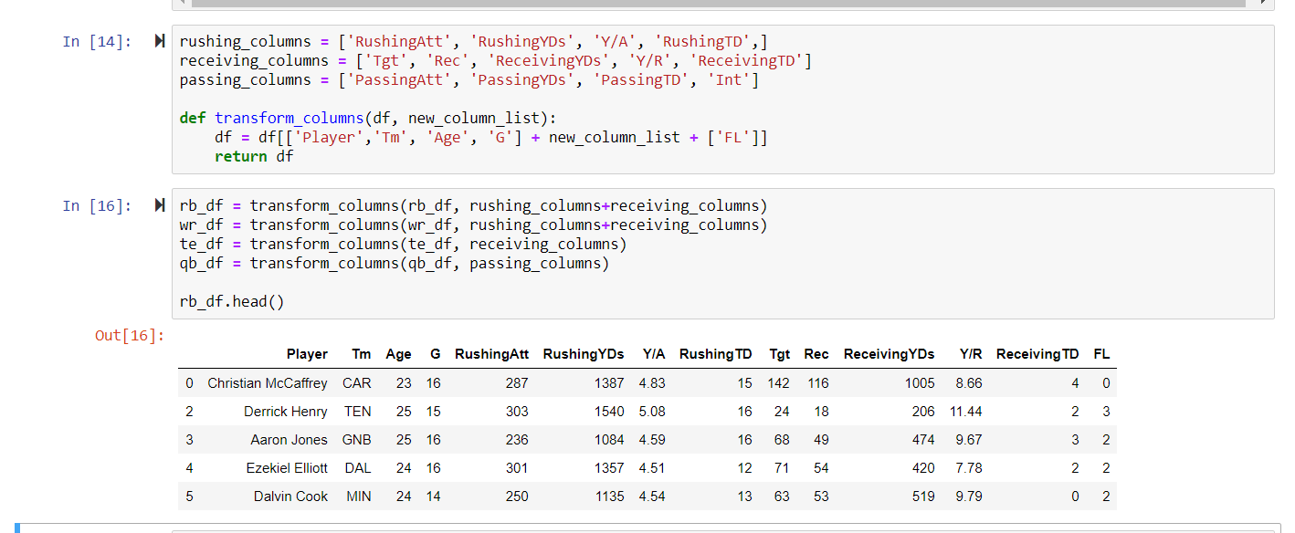
Our Second Block of Code
This first cell looks kind of complicated but it’s really not. What we are doing here is
essentially assigning columns to the different DataFrames. Although trick plays happen where running backs and
wide receivers sometimes throw the ball, this is not something we can ever predict, so we can exclude those
columns from our wr_df and rb_df for the sake of simplicity. The syntax for filtering
DataFrames and creating new ones based on desired column names is df = df[[‘ColumnName1’,
‘ColumnName2’,]]
I wrote a little function to make the code more legible and simplistic. But essentially we
are concatenating lists and following the syntax shown above. All players should have a fumble column, but it’s
kind of miscellaneous stat that’s hard to predict so we leave it at the end (Unless your name is Daniel Jones –
then we know you’re going to fumble). Our function returns a new DataFrame, and we assign it to a new variable.
You’re welcome to skip this whole step if you want to include every column (as tight-ends do run the ball
sometimes and wide receivers do sometimes pass the ball).
At the end, we run rb_df.head() to see our new DataFrame. We will be working
with the rb_df for the remainder of the post for the sake of brevity, but you are welcome to run
these data visualizations on any of the created DataFrames.
So now that we have our DataFrame ready, we can start to use pandas to answer some fantasy
football questions. One maxim I followed this year when deciding on draft picks, waiver-wire pickups, and
sit-start decisions was usage is king. Unless his name was Aaron Jones, I avoided running back
committees at all cost. This maxim becomes more and more obvious the more you play fantasy, but the temptation
to start the Will Fuller’s and Sammy Watkin’s of the fantasy world are forever present (Against my better
judgement, I still started Will Fuller Week 16 against Tampa Bay, oops).
But let’s not just rely on intuition, as our intuition is sometimes wrong. Let’s try to
answer the question –
“What is more correlated to fantasy performance for running backs, usage or
efficiency?”
Our Third Block of Code - Plotting Our DataFrame
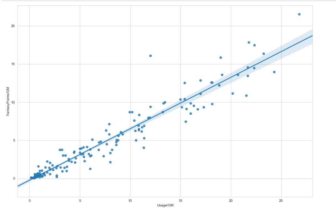
Below is the code for plotting a graph of usage (the x-axis) versus fantasy points per game (the
y-axis)
The resulting graph is show below. No surprises here, usage and fantasy points per game are heavily
correlated.
Let’s break down the code step by step again.
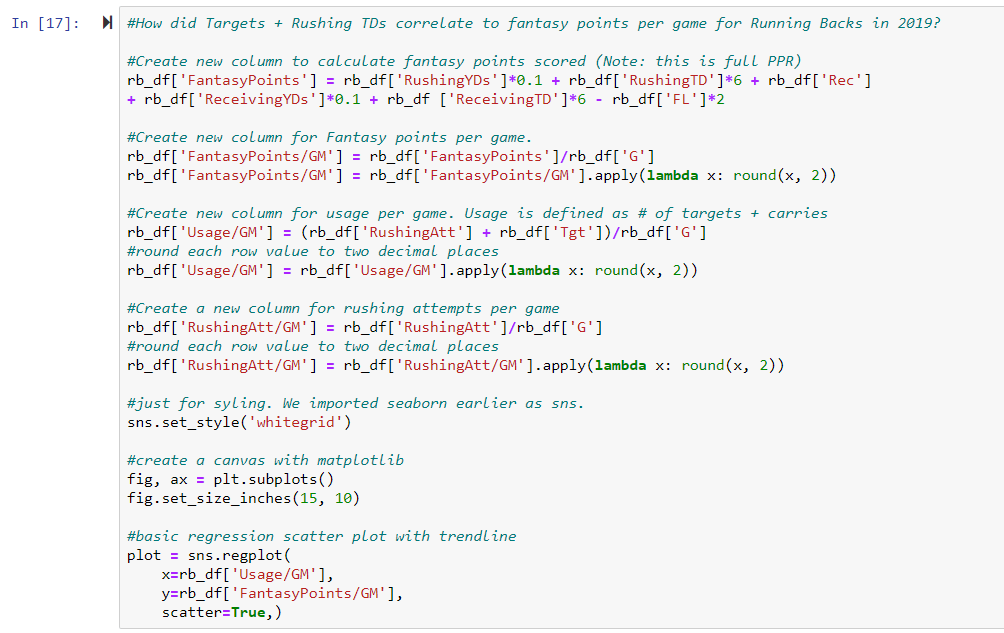
rb_df['FantasyPoints'] = rb_df['RushingYDs']*0.1 + rb_df['RushingTD']*6 + rb_df['Rec'] + rb_df['ReceivingYDs']*0.1 + rb_df
['ReceivingTD']*6 -
rb_df['FL']*2
We can create a new column with pandas based off the value of other columns by doing
df[“New column name” = df[“other column”] + …
Here, we want to create a column that calculates total fantasy points. We used 0.1 points
per rushing yard + 6 points per rushing TD + 1 point per reception + 0.1 points per receiving yard + 6 points
per receiving TD – 2 points per fumble lost.
You’re welcome to change the weighting of points per reception to 0.5 if you play in a
0.5PPR league or remove it altogether if you use standard.
#Create new column for Fantasy points per game.
rb_df['FantasyPoints/GM'] = rb_df['FantasyPoints']/rb_df['G']
rb_df['FantasyPoints/GM'] = rb_df['FantasyPoints/GM'].apply(lambda x: round(x, 2))
We essentially did the same thing here. We created a new column based off a previous
column, and then used the .apply() built-in method and a lambda function to round each answer to
two decimal places.
#Create new column for usage per game. Usage is defined as # of targets + carries
rb_df['Usage/GM'] = (rb_df['RushingAtt'] + rb_df['Tgt'])/rb_df['G']
#round each row value to two decimal places
rb_df['Usage/GM'] = rb_df['Usage/GM'].apply(lambda x: round(x, 2))
Same thing here. We created a new column for “Usage/GM”. We defined usage as number of
targets + number of carries. I like to use targets and not catches for analyzing players. I believe targets are
a better measure of usage, and you should prioritize players who are seeing an increasing number of targets and
target share. But that’s a whole different discussion.
#just for styling. We imported seaborn earlier as sns.
sns.set_style('whitegrid')
#create a canvas with matplotlib
fig, ax = plt.subplots()
fig.set_size_inches(15, 10)
#basic regression scatter plot with trendline
plot = sns.regplot(
x=rb_df['Usage/GM'],
y=rb_df['FantasyPoints/GM'],
scatter=True,)
There’s a bit of magic happening here and I don’t want to delve to deep into this for the
sake of the brevity of this post. Check out the documentation for seaborn and matplotlib/pyplot here. But essentially, we are just setting styling with
sns.setstyle(). A list of possible arguments for setstyle() can be found in the
seaborn docs. What we are doing with plt.subplots() is essentially creating a canvas to plot our
graphs. We then use fig.set_figure_inches(15, 10) to set the height and width of our “canvas”.
That’s all you really need to know for now. And finally, we plot using seaborn and the regplot function, using
the “Usage/GM” column as our x-axis and [“FantasyPoints/GM”] as our y-axis. Finally we
set scatter = True to tell seaborn we want a scatter plot – and voila, our graph renders.
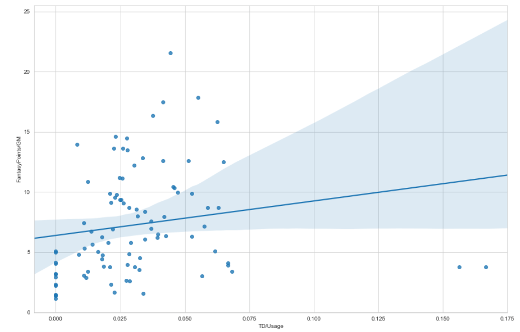
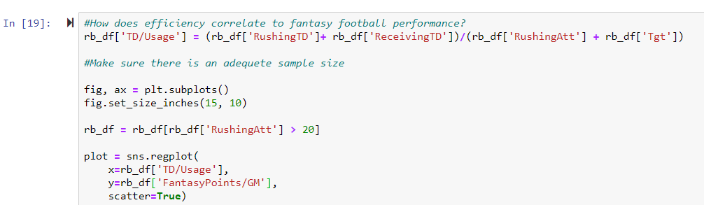
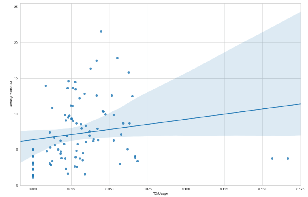
Our Fourth Block of Code - Efficiency vs. Fantasy Points per Game
Below is the code evaluating the correlation between efficiency and fantasy points per game.
As you can see below, efficiency is not nearly as strongly correlated as usage. We expected this,
but the comparison of the two graphs confirms how much more important prioritizing usage is if you want to win
your fantasy football league.
Let’s break this additional code down briefly.
rb_df['TD/Usage'] = (rb_df['RushingTD']+ rb_df['ReceivingTD'])/(rb_df['RushingAtt'] + rb_df['Tgt'])
fig, ax = plt.subplots()
fig.set_size_inches(15, 10)
rb_df = rb_df[rb_df['RushingAtt'] >
20]
plot = sns.regplot(
x=rb_df['TD/Usage'],
y=rb_df['FantasyPoints/GM'],
scatter=True)
We are creating a new column again based off other columns, so the syntax is very similar
to our previous graph. We define efficiency as TD’s per usage. I admit there are probably better measures of
efficiency, but for simplicity’s sake, let’s just roll with this one. I actually decided on this measure because
I drafted Aaron Jones and struggled with making the decision of whether to hold on to him or trade him for
someone more consistent (I decided to hold on to him). Aaron Jones is the textbook definition of efficient. He’s
part of a running back committee, yet somehow was top 5 in touchdowns almost all year.
Anyways, the setup for matplotlib is the same, we use plt.subplots() to create
our “canvas”, and seaborn is essentially the same but we are using a different x and y axis. The one main
difference here is that we are filtering for minimum rushing attempts. Remember when we filtered based off
position to create our separate DataFrames? We are essentially doing the same thing here, but we are using a
> operator and setting a minimum of 20 carries based off the RushingAtt column.
Takeaways
The main takeaway from all this should be to draft, pick up, start your running back
workhorses. When you see players on the waivers seeing an increasing trend of targets and carries, pick them up.
Don’t start running backs until they have proven that they are going to be heavily utilized in the offense (Mike
Boone hype train anyone?).
This was a pretty basic analysis and in future posts we’ll dive deeper into using Python to help you
win your league next year and crush the 2020 draft. I hope you all enjoyed this and this sends you down a rabbit
hole of sports analytics! If you have any questions comment below, I’ll be sure to help out.
Check out
part two of the series here.