If you have any questions about the code here, feel free to reach out to me on Twitter or on Reddit.
Shameless Plug Section
If you like Fantasy Football and have an interest in learning how to code, check out our Ultimate Guide on Learning Python with Fantasy Football Online Course. Here is a link to purchase for 15% off. The course includes 15 chapters of material, 14 hours of video, hundreds of data sets, lifetime updates, and a Slack channel invite to join the Fantasy Football with Python community.
Hi all, in this part of the intermediate series, I'm going to take you throw a project we go through in my course I offer on this site - only this post is updated for the most current season. In the course, I offer a more in-depth analysis of this project (albeit applied to the 2019-2020 season) along with an hour long video explanation.
Some of you may have noticed it's been a while since I've posted, but I'm hoping to ramp up new content leading in to the new season.
The project
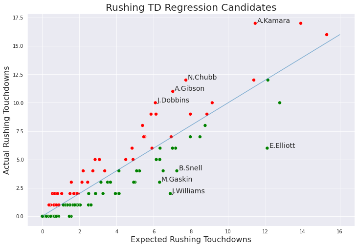
We are going to be doing a TD regression analysis for RBs. Essentially, for each RB this season, we'll be looking at their number of carries + how far each carry was from the endzone. Based off how far a player received a carry from the endzone, we'll assign a score or expected touchdown value to their carry based off historical numbers on how probable a TD is from that given yardline. Once you add each carry's expected TD value for each RB, you'll get an expected TD number for the entire season. For each RB, we'll be comparing that expected TD value to the actual TD values they posted. If a player actually scored more TDs than their expected TD value, we'll say they are due for negative regression and "over performed" their season. And vice versa if their expected TD value was higher than their actual TD posting.
I've posted this type of analysis on Reddit previously and got absolutely roasted for it. There were some problems with the original analysis, and I've decided to take suggestions from Redditors who brought up some unique solutions. The problem with the analysis I proposed in the paragraph above is that theoretically a RB could end up having a greater than 1 expected touchdown on a drive, especially if they received multiple goal line carries on a given drive. This obviously doesn't make sense - the workaround to this problem is to cap expected touchdowns to 0.99 or 1 per drive.
No analysis is perfect - obviously some RBs have that special ability to break off a 60 yard TD at any moment, while other RBs simply do not. Those RBs that have that special ability to break off a huge play at any moment obviously have a higher probability of scoring a TD per handoff than an average RB. Thus, those RBs will be underweighted using this sort of analysis. Conversely, RBs that don't have that special ability are overweighted by this sort of analysis. Even though I run Fantasy Football DATA Pros, I advocate for using quantative and qualitative measures in all of your analysis. Fantasy Football is part art, part science, and data never tells the full story.
If you have any suggestions for improving the analysis further, please say so in the reddit comments.
The code
With that out of the way, let's start work on the project. You'll need to run this code in a notebook environment, for those unfamiliar with my content, and the easiest solution would be to set up a Google Colab runtime.
To start, we're going to be installing the nflfastpy library which I personally maintain. It pulls from the nflfastR data package and exposes 20 years of play by play data.
Importing our libraries as always, and setting the style for our visualizations.
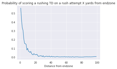
In this first block of code, we are going to be pulling data from the past 5 years of the NFL, excluding the most recent season and concatenating the data together into one big DataFrame. We will be using this data to find the probability of scoring a touchdown X yards from the endzone, for each value of X 0 - 100, and putting this all in to a DataFrame we'll call rushing_df_probs.
Now we're going to take our big DataFrame and transform it the way I described. Like I said earlier, this post will not be as in depth as my course, so if the code here confuses a bit, it's covered a bit more in depth in the course. I've added some comments to each line to explain what we're doing.
|
yardline_100 |
probability_of_touchdown |
| 0 |
1.0 |
0.560390 |
| 3 |
2.0 |
0.428058 |
| 5 |
3.0 |
0.336910 |
| 7 |
4.0 |
0.304251 |
| 9 |
5.0 |
0.206349 |
Now we can plot our DataFrame you see above so we can visualize the probability of scoring a rushing touchdown X yards from the endzone. As anyone could have expected, as you get farther from the endzone, the less probable it is a TD will occur. We're more concerned with the values from the DataFrame and using it it calculate expected TDs than any sort of revelation from visualizing this data.
Now we'll load in 2020 data. We're going to use the rushing_df_probs DataFrame to calculate expected TD values for each RB in the 2020 season, then compare that calculated value to actual TDs scored.
We'll also load in roster data for 2020, since by default play by play data will not contain the position for a rushing/receiving/passing player. We want to only include RBs in this analysis, so this step is important. Here, we'll filter out our roster DataFrame to only include RBs, grab the player ids for all RBs, and then filter our 2020 data to only include the player ids located from our roster DataFrame. While play by play data doesn't provide us with positions, it does provide us with player ids for the rushing/receiving/passing player on each play.
Below, we're going to filter, clean, and merge our data a bit. I've added comments above each operation.
|
rusher_id |
drive_id |
rusher_player_name |
rush_attempt |
rush_touchdown |
yardline_100 |
probability_of_touchdown |
| 0 |
00-0031687 |
2020_01_ARI_SF_1 |
R.Mostert |
1.0 |
0.0 |
55.0 |
0.003171 |
| 1 |
00-0031687 |
2020_01_ARI_SF_1 |
R.Mostert |
1.0 |
0.0 |
41.0 |
0.010914 |
| 2 |
00-0031687 |
2020_01_ARI_SF_1 |
R.Mostert |
1.0 |
0.0 |
39.0 |
0.002841 |
| 3 |
00-0031687 |
2020_01_ARI_SF_5 |
R.Mostert |
1.0 |
0.0 |
64.0 |
0.000939 |
| 4 |
00-0033118 |
2020_01_ARI_SF_8 |
K.Drake |
1.0 |
0.0 |
78.0 |
0.001383 |
Now, we have a DataFrame that contains each rush attempt for the season by an RB, with each play assigned an expected touchdown value. All that's left to do now is to group by rusher id and add up the actual touchcowns and the expected values, right? Recall in the beginning of this post we discussed the problem I originally ran into when running this sort of analysis. Some RBs would receive a greater than 1 value for expected TDs on a given drive, which made no sense. So, we need to limit expected TDs to 1 per drive, or at the very least, very close to 1. That was the reason for assigning a drive id column above. First, we will add expected values for each RB, drive without this cap.
We can see here we have 48 instances where an RB was assigned a expected TD value of greater than 1 on a single drive. Let's cap all drives to 0.999.
Now that we've gotten that out of the way, let's groupby again and this time only group by rusher id. We'll assign a column called positive_regression_candidate which will flash True when expected touchdowns > actual touchdowns, indicating a player may be due for positive regression. The delta column we assign here will be the difference expected and actual touchdowns.
|
rusher_id |
rusher_player_name |
actual_touchdowns |
expected_touchdowns |
positive_regression_candidate |
delta |
| 57 |
00-0033893 |
D.Cook |
16.0 |
15.298370 |
False |
0.701630 |
| 36 |
00-0032764 |
D.Henry |
17.0 |
13.904407 |
False |
3.095593 |
| 43 |
00-0033118 |
K.Drake |
10.0 |
12.773619 |
True |
2.773619 |
| 115 |
00-0035700 |
J.Jacobs |
12.0 |
12.135000 |
True |
0.135000 |
| 42 |
00-0033045 |
E.Elliott |
6.0 |
12.099989 |
True |
6.099989 |
All that's left now is to visualize the results, but I encourage you to mess around with this data because it's interesting and useful on it's own. I've added some comments to the code below to guide you through it once again.
That's all for this post. Thank you for reading, you guys are awesome!
 Photo by Jerome Miron, USA TODAY Sports