Learn Python with NFL Data: Evaluating Team Strength with EPA (Part 2)

Learn how to use Python to evaluate team strength using nflfastR's EPA model.
Learn how to use Python to evaluate team strength using nflfastR's EPA model.
This post is a continuation of the last post focused on general NFL-analytics using NflFastPy's EPA model.
The code below will build heavily on the last post so if you'd like to follow along the code it may be necessary to go back and start with the blog post from last week. Last week we used NflFastPy's EPA (Estimated Points Added) model to visualize the best offenses and defenses in the league. Now we will use that information along with schedule data to look at the fantasy fallout.
NflFastPy's play by play data comes with EPA data for each play. EPA is a model that estimates the expected points added per individual play based on starting and ending field position, down, and field goal distance.
Each play has an EPA, and we're going to be finding each team's EPA per play on offense and defense. For offense, it's straight forward. If a play has an EPA of 1.2 on offense, that means the offense moved the ball such that they added an expected 1.2 points to their score. For defense, it's going to be the opposite. If a team is on defense, and the EPA for the play is 1.2, then we'll say the defense gave up or allowed an estimated 1.2 points on the play. Team defenses with more negative EPAs are better defenses, while team defenses with more positive EPAs are worse defenses.
Now that we know the offensive and defensive value of each team we can see how hard a team's schedule has been so far and how hard it will be for the rest of the season. By doing this we are essentially normalizing a team's performance and evaluating with the opposition strength in mind. By looking at the biggest change in schedule strength we can zero in on fantasy players on teams that will have a much easier schedule. We can also fade some players that have performed well so far this year but is about to face some tough teams.
This analysis is very helpful in putting fantasy performances into perspective. I often use it to evaluate current value versus future value which gives an edge when it comes to trading.
Let's get to the code. First things first, load up your Google colab or jupyter notebook and import the libraries we'll need for this post.
Next, we'll load in 2021 play by play data via NflFastPy. We've used this data quite a bit, just as a reminder it is an extensive database detailing every snap that has taken place so far this year.
| play_id | game_id | old_game_id | home_team | away_team | season_type | week | posteam | posteam_type | defteam | ... | out_of_bounds | home_opening_kickoff | qb_epa | xyac_epa | xyac_mean_yardage | xyac_median_yardage | xyac_success | xyac_fd | xpass | pass_oe | |
|---|---|---|---|---|---|---|---|---|---|---|---|---|---|---|---|---|---|---|---|---|---|
| 0 | 1 | 2021_01_ARI_TEN | 2021091207 | TEN | ARI | REG | 1 | NaN | NaN | NaN | ... | 0 | 1 | NaN | NaN | NaN | NaN | NaN | NaN | NaN | NaN |
| 1 | 40 | 2021_01_ARI_TEN | 2021091207 | TEN | ARI | REG | 1 | TEN | home | ARI | ... | 0 | 1 | 0.000000 | NaN | NaN | NaN | NaN | NaN | NaN | NaN |
| 2 | 55 | 2021_01_ARI_TEN | 2021091207 | TEN | ARI | REG | 1 | TEN | home | ARI | ... | 0 | 1 | -1.399805 | NaN | NaN | NaN | NaN | NaN | 0.491433 | -49.143299 |
| 3 | 76 | 2021_01_ARI_TEN | 2021091207 | TEN | ARI | REG | 1 | TEN | home | ARI | ... | 0 | 1 | 0.032412 | 1.165133 | 5.803177 | 4.0 | 0.896654 | 0.125098 | 0.697346 | 30.265415 |
| 4 | 100 | 2021_01_ARI_TEN | 2021091207 | TEN | ARI | REG | 1 | TEN | home | ARI | ... | 0 | 1 | -1.532898 | 0.256036 | 4.147637 | 2.0 | 0.965009 | 0.965009 | 0.978253 | 2.174652 |
5 rows × 372 columns
Here, we're making a DataFrame called epa_df which will sum up team EPAs for each play and we'll also count the number of plays. Using this we calculate epa per play. Then we rinse and repeat to add in the defensive epa.
| offense_epa | offense_plays | offense_epa/play | |
|---|---|---|---|
| KC | 83.132330 | 875 | 0.095008 |
| BUF | 55.972040 | 767 | 0.072975 |
| TB | 52.091916 | 763 | 0.068272 |
| IND | 50.963161 | 830 | 0.061401 |
| DAL | 49.035640 | 807 | 0.060763 |
These are the 5 best offenses in the league by EPA per play. Its always good practice to check your results and confirm they are what you expect, or at least make sense. The 5 teams listed above are considered some of the best offenses in the league so this checks out.
| offense_epa | offense_plays | offense_epa/play | defense_epa | defense_plays | defense_epa/play | |
|---|---|---|---|---|---|---|
| NYJ | -63.920613 | 754 | -0.084775 | 97.753149 | 770 | 0.126952 |
| DET | -74.370818 | 767 | -0.096963 | 59.751196 | 724 | 0.082529 |
| WAS | -16.072293 | 740 | -0.021719 | 54.860977 | 745 | 0.073639 |
| KC | 83.132330 | 875 | 0.095008 | 52.167113 | 791 | 0.065951 |
| HOU | -106.693127 | 713 | -0.149640 | 42.932640 | 735 | 0.058412 |
These are the 5 worst defenses in the league by EPA per play. Remember, more positive EPAs per play on the defense side are bad. This means the defense is allowing (an estimated amount) of more points per play.
Now we can utilize the information created above in addition to schedule data to get some valuable insights. Most of this code is definitions, transformations, and manipulations. I'll breeze through it fairly quickly, but feel free to reach out if you have specific questions.
First we grab schedule data for all of 2021, and then define a function to extract all opponents for a singular team. Then we associate the EPA's for each list of opponents. And lastly, input the number of weeks played in the season to see the EPA of offenses and defenses already faced compared to the teams the rest of the season.
Now we can use the definitions from above to populate a dataframe with all the EPA information.
| Team | Offense_EPA_Delta | Defense_EPA_Delta | |
|---|---|---|---|
| 3 | BUF | 0.032660 | -0.074916 |
| 13 | IND | 0.017576 | -0.061019 |
| 21 | NE | 0.034564 | -0.036731 |
| 1 | ATL | 0.004538 | -0.035490 |
| 29 | TB | -0.025732 | -0.030051 |
Let's interpret the numbers. A positive offensive delta means a team will be facing better offenses in the second half of the season than the first half. A positive defensive delta means a team will be facing worse defenses in the second half of the season than the first half. So in the dataframe above sorted by defensive EPA delta we can see 5 teams that are jumping from easy schedules to hard schedules (denoted by a negative defense EPA delta). These are teams you may want to avoid when streaming players.
Now lets make a similar plot to last post. This time we will plot the delta epa for offense and defense. This metric is effectively the change in strength of schedule from the first half to the second half of the season (for both offense and defense separately).
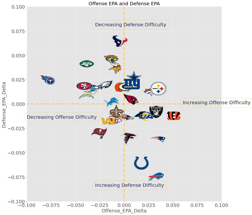
The best Way to interpret this plot is to look at the x or y axis one at a time. Lets start with the x axis.
The x axis contains information about opposing offenses. If a team is to the right of the origin the team will be playing better offenses in the second half than they did in the first half. If a team is to the left of the origin the team will be playing worse offenses in the second half than they did in the first half. A couple notable teams are the Titans and the Raiders. The Titans played some really great offensive teams in the first half including Cardinals, Chiefs, Bills, Rams, and the Colts twice. In the second half they will face the Jaguars, Dolphins, Steelers, and the Texans twice. So it makes sense we see them pretty far on the left side of the plot since they will be facing easier offenses. This means the Titans defense could be a great pick up down the stretch. The Raiders on the other hand will be facing better offenses. This is valuable information since if you believe the Raiders will get into some shoot outs to keep up with their opponents, Derek Carr is worth monitoring from a fantasy perspective.
The y axis contains information about opposing defenses. If a team is above the origin the team will be playing worse defenses in the second half than they did in the first half. If a team is below the origin the team will be playing better defenses in the second half than they did in the first half. The Bills for example will be facing much better defenses in their final 8 games. They face off against the Saints, Panthers and the Patriots twice. All of these teams are top 10 defenses according to Pro Football Reference. It is also interesting to note the Bills play the Jets (possibly the worst defense in the league) in week 18 and this is baked into our analysis. If you do not play week 18 in your fantasy football leagues then you don't get the points from this easy match up. If you are interested I recommend playing with this analysis and cutting off week 18 to get more specific results for your fantasy football leagues.
As a final note I'd like to add that this analysis does not take into account a couple things. First off, we are looking specifically at how teams have performed in the first half of the season and assuming their performance will be similar in the future. This doesn't account for future injuries (or players returning), home / road splits, or if a team is on a hot streak. Like I mentioned before this is a helpful analysis when trying to evaluate players performances so far this season and if their schedule will lighten up the rest of the way.
I'll leave the full list of defensive EPA deltas below. Thanks for reading!
| Offense_EPA_Delta | Defense_EPA_Delta | |
|---|---|---|
| Team | ||
| BUF | 0.032660 | -0.074916 |
| IND | 0.017576 | -0.061019 |
| NE | 0.034564 | -0.036731 |
| ATL | 0.004538 | -0.035490 |
| TB | -0.025732 | -0.030051 |
| WAS | -0.016768 | -0.017858 |
| KC | -0.010037 | -0.016972 |
| BAL | 0.002009 | -0.014294 |
| LA | 0.022284 | -0.013198 |
| CIN | 0.050457 | -0.012448 |
| CAR | 0.017572 | -0.011302 |
| CHI | -0.007382 | -0.010194 |
| LV | 0.032828 | -0.008129 |
| NO | -0.008228 | -0.007803 |
| DET | -0.013554 | 0.002108 |
| ARI | 0.006472 | 0.004757 |
| LAC | -0.038776 | 0.007439 |
| DEN | 0.028261 | 0.011700 |
| MIA | -0.033951 | 0.014193 |
| PIT | 0.034952 | 0.015708 |
| SEA | -0.033785 | 0.017025 |
| CLE | -0.002370 | 0.017172 |
| GB | 0.001488 | 0.017510 |
| SF | -0.041011 | 0.018394 |
| PHI | -0.019668 | 0.019391 |
| NYG | 0.007705 | 0.020212 |
| TEN | -0.079209 | 0.024465 |
| DAL | 0.010094 | 0.027720 |
| MIN | -0.009664 | 0.037633 |
| NYJ | -0.038668 | 0.041142 |
| JAX | -0.013211 | 0.045372 |
| HOU | -0.004387 | 0.064132 |