Learn Python with NFL Next Gen Data: Jamal Agnew
Learn how to use Python to analyze Next Gen Punt Return Stats.
Learn how to use Python to analyze Next Gen Punt Return Stats.
In this post we're going to take another look at NFL Next Gen Stats. I wrote the previous post focused on it and we'll be looking at it for one more week. As I mentioned before, this dataset is very vast and there are many interesting football and fantasy football applications. You just need an idea to get started!
Last post we looked at Zeke's rushing in 2018. There is some field level data I walk through as well as take a look at how Zeke fairs against different number of defenders in the box. In this post we'll take the field data a step further and look at movement data on punt returns for Jamal Agnew. Once again, this dataset was very large to start, so I decided to narrow the scope of the notebook to focus on a single player and play type. I hope this allows you guys to get up and running and apply it to new ideas on your own!
Let me explain what I mean when I say we are going to be looking at movement data. NFL Next Gen Stats uses cameras and player trackers so they actually have access to precise locations of every player on the field and every moment. So in our dataset each row is a specific play, player, and moment in time on that play. Each moment the data is recorded is separated by 0.1 seconds. So for example if Jamal Agnew returns a punt for 20 yards and it took him 3 seconds to do so there will be 30 rows of data to describe that play. We are going to take that information and tie it all together to get a complete picture of where Jamal Agnew is on the field every 0.1 seconds.
To start, let's import our standard libraries in Google Colab or your locally hosted jupyter notebook.
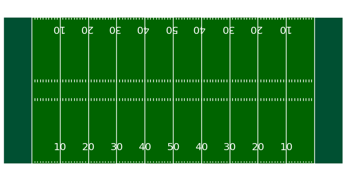
Next we have to import the football field that we will be plotting on. This was used in the previous post and instead of writing all the code again (it was pretty lengthy), I am going to write that code in a separate file and pull the function from it. To do this we use a handy package, ipynb, which allows us to access other jupyter notebooks inside our file system and access code, functions, classes in another notebook. This saves a ton of time and it helps clean up notebook by putting lengthy helper functions elsewhere.
After ipynb you write fs to denote file system, and then defs to denote the functions defined in the notebook (full denotes the entire notebook). Then follow that with the notebook name, and finally import the specific function desired.
If you want more details about how this field is created head over to my last post where I show the entire code. Let's see our football field!
Next, let's load the data source from a csv I saved earlier. The original data was so large I extracted only the plays in which Jamal Agnew was returning punts.
| time | x | y | s | a | dis | o | dir | event | nflId | displayName | jerseyNumber | position | team | frameId | gameId | playId | playDirection | |
|---|---|---|---|---|---|---|---|---|---|---|---|---|---|---|---|---|---|---|
| 0 | 2021-01-03T18:02:34.200 | 76.17 | 34.91 | 0.28 | 0.86 | 0.02 | 265.67 | 281.62 | None | 44978.0 | Jamal Agnew | 39.0 | WR | home | 1 | 2021010305 | 40 | left |
| 1 | 2021-01-03T18:02:34.300 | 76.14 | 34.91 | 0.36 | 0.77 | 0.04 | 264.88 | 286.88 | None | 44978.0 | Jamal Agnew | 39.0 | WR | home | 2 | 2021010305 | 40 | left |
| 2 | 2021-01-03T18:02:34.400 | 76.12 | 34.92 | 0.32 | 0.42 | 0.02 | 260.03 | 289.38 | None | 44978.0 | Jamal Agnew | 39.0 | WR | home | 3 | 2021010305 | 40 | left |
| 3 | 2021-01-03T18:02:34.500 | 76.10 | 34.94 | 0.30 | 0.33 | 0.02 | 262.51 | 306.40 | None | 44978.0 | Jamal Agnew | 39.0 | WR | home | 4 | 2021010305 | 40 | left |
| 4 | 2021-01-03T18:02:34.600 | 76.08 | 34.96 | 0.31 | 0.28 | 0.03 | 261.19 | 311.23 | None | 44978.0 | Jamal Agnew | 39.0 | WR | home | 5 | 2021010305 | 40 | left |
What's nice about the football field I created is that the dimensions lineup with our dataset. This means you can plot a player's (X,Y) coordinates and it would be correctly plotted to scale. The dataset also records s (speed yards/s), a (acceleration yards/s2), dis (distance traveled since previous recorded point in yards), dir (angle of player motion). These are the main features I was concerned with, but feel free to explore the many others and reach out if you have any clarifying questions.
Take notice to the time column and how each row is separated by 0.1 seconds like I mentioned in the introduction. Using (X,Y) coordinates and speed we can create a pretty cool plot that shows Jamal returning a punt with his position on the field and speed every 0.1 seconds during the play. We'll be focusing on individual punt returns and if you want to try it out on your own I'll leave some play ID's for you to use. Let's check it out!
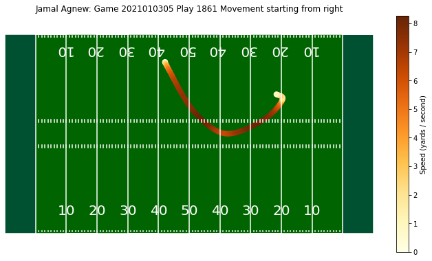
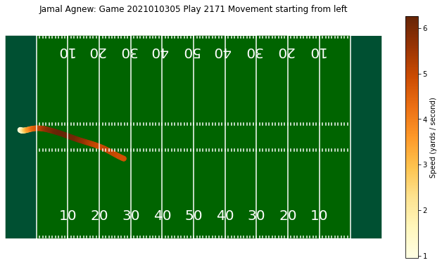
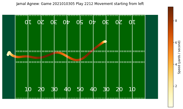
I thought these plots turned out pretty good. It is clear exactly where Agnew started, finished, and how fast he went. It looks like it takes him a few seconds to get up to speed and then he stays consistent after that. These plots are about as much information you can possible extract from a play. It's just one step below actually watching the tape. I tried looking at all of Jamal Agnew's returns together to see if there were any trends I could pick up, but the plot got a bit messy. I hope you enjoy this NFL style analysis and next week we will be getting back into the fantasy side of things.